An approach to estimate carbon stocks change in forest carbon pools under the UNFCCC: the Italian case
iForest - Biogeosciences and Forestry, Volume 1, Issue 2, Pages 86-95 (2008)
doi: https://doi.org/10.3832/ifor0457-0010086
Published: May 20, 2008 - Copyright © 2008 SISEF
Research Articles
Abstract
Under the UNFCCC, Annex I Parties must report annually a National GHG Inventories of anthropogenic emissions by sources and removals by sinks. LULUCF is one of the six sectors of the inventory: in this sector any emissions and removals of GHGs by land management should be reported, included the large GHGs fluxes generated by forest management and land-use changes into and from forest. In this context every Party has to produce a proper model in order to be able to fulfil GHGs Inventory request for forest sector. Taking Italy as a study case, the paper aims at presenting a new methodology for updating stock changes for years between national forest inventories, in order to reproduce annual stock changes in the five UNFCCC forest carbon pools, following the UNFCCC requirements in the context of carbon reporting.
Keywords
Carbon stock, GHG inventory, LULUCF, Yield model, Sink, C pools
Introduction
Under the United Nations Framework Convention on Climate Change (UNFCCC) each industrialised country listed in Annex I of the Convention must report annually a National Greenhouse Gas Inventory of its anthropogenic emissions by sources and removals by sinks of greenhouse gases (GHGs) not controlled by the Montreal Protocol.
One out of six sectors of the inventory concerns Land Use, Land-Use Change and Forestry categories (LULUCF). In this sector any emissions and removals of GHGs by managed land should be reported. Among land uses, forest land use is one of the most relevant, due to large carbon pools and associated large GHGs fluxes generated by forest management and land-use changes into and from forest.
Interrelations between forest and climate system have been a major focus of research since mid-1980s. Up to date, several models have been developed that analyze and simulate carbon budgets and fluxes at level of forest stands. These tools range from very detailed models based on ecophysiological processes and driven by environmental parameters (e.g., [36]) to very general empirical, descriptive models of carbon budgets within forest stands (e.g., [29]). None of these models have been widely used for operational application, and none of them has been adopted as standard for carbon reporting under UNFCCC. As the main reason for this we consider the age dependency of all these models in which all stand variables being driven by the age of the forest/plantation. In reality, however, growth is strictly related to species and to local environmental conditions. In this respect the most realistic estimates of carbon stock changes have to be derived by yield models, whose input data are directly connected with National Forest Inventories (NFI). UNFCCC requirements in the context of carbon reporting also require a series of features for forest sector which are only compatible with yield models. Under current UNFCCC reporting guidelines ([16], [17]) estimates of carbon stock changes in the forest sector must still be based on national forest inventories and yield models. In this context every Country is encouraged to produce a proper national model in order to be able to annually fulfil GHG’s Inventory request for the forest sector.
To be utilized for UNFCCC reporting the model shall respond to some characteristics:
- it shall be based on: (i) official statistical data like the National Forest Inventory and national forest statistics; (ii) peer reviewed scientific dataset;
- it shall produce annual carbon stock changes in each carbon pool;
- it shall be accurate and, in the Kyoto Protocol perspective, conservative (i.e., neither overestimate increases nor underestimate decreases in carbon stocks in carbon pools).
A general complication for UNFCCC carbon reporting in the forestry sector is connected to the need of annual reporting since 1990, whereas NFI’s are performed in cycles of 5-10 years in some countries with best case of NFI data availability. In Italy, for example, there is a NFI available for the year 1985 and a new NFI is still ongoing. Anyway, considering the timing of NFIs, there is the need of reporting carbon stock changes for any year between consecutive inventories with a reliable methodology, based on growth relationships and annually measured forest parameters, rather than a simple extrapolation between years.
Following the above rationale, we propose a new methodology, which is based on existing NFI data for 1985 and new forest area estimates from the ongoing NFI, in order to reproduce annual stock changes in the five UNFCCC forest carbon pools ([17]). Taking Italy as an example, the paper aims at presenting a methodology for updating stock changes for years between national forest inventories, which could eventually be used also for other countries with similar data availability (Tab. 1).
Tab. 1 - Forest areas from 1985 to 2006.
| Year | Forest area (kha) |
|---|---|
| 1985 | 8675 |
| 1986 | 8793 |
| 1987 | 8908 |
| 1988 | 9028 |
| 1989 | 9145 |
| 1990 | 9263 |
| 1991 | 9380 |
| 1992 | 9498 |
| 1993 | 9616 |
| 1994 | 9733 |
| 1995 | 9851 |
| 1996 | 9968 |
| 1997 | 10086 |
| 1998 | 10203 |
| 1999 | 10321 |
| 2000 | 10438 |
| 2001 | 10556 |
| 2002 | 10674 |
| 2003 | 10791 |
| 2004 | 10909 |
| 2005 | 11026 |
| 2006 | 11144 |
The For-est (Forest Estimates) Model
In forest science, estimates of the current increment has always been related with age of forest stand (as in yield tables) in order to define the proper rotation period, which depends on age and productivity of the stand. Age could be the best parameter for productivity assessment of single trees, but it is not always appropriate for estimates at the stand level. This is particularly true for natural stands, where forest dynamics is driven by optimised use of natural resources, which includes tree mortality and natural regeneration in gaps. These processes result in a complex mosaic of different ages or cohortes; under these conditions the use of age dependant relationships for productivity estimations is not always appropriate.
The type of forest management outlined above is especially common in Mediterranean countries, where even-aged stand is not the rule. Correspondingly, Garcia ([13]) writes: “The use of age on the right-hand-side (as independent variable) is conceptually unsatisfactory in that, at least in the sense of elapsed time t, it does not have a physical presence (other than as a number of growth rings), and therefore should not be given a causal meaning. Actually, when foresters say age they often think size.”
Lähde et al. ([23]) made an analysis on the relation between variables for various forest structures and compositfions, showing a higher correlation between current increment and growing stock compared to current increment and age.
There are various studies showing a relation among dimensional attributes of trees without considering the age ([31], [38], [35], [11], [12], [34], [3], [6], [7], [8], [24], [2], [37], [9], [25], [30]). For instance, Chrimes ([4]) demonstrates that current increment is directly and significantly related to volume.
Thrower ([35]) formulated an equation that calculates current increment as a function of growing stock and of Potential Site Index (PSI) considering this as a variant of the Langsaeter curve, which consists in a univocal relation between stand density and current increment ([26]).
For these reasons, and because of the large majority of Italian forest are not even-aged, we propose to use an approach based on growth curves not dependant on age but considering the growing stock as independent variable and the current increment as dependent one.
We further propose that all carbon stocks in carbon pools shall be estimated in function of the growing stock. This is an advantage compared to other approaches since the growing stock is closely related with other carbon budget components such as soil carbon, litter, deadwood etc. and it is a unique driver, simply assessable, widely and iteratively sampled on national territory (by NFIs). Moreover, growing stock data could be verified using independent dataset as regional forest inventories and/or local forest management plan.
In order to calculate current increment as a function of growing stock the Richards function ([33]) has been selected. Based on a biologically realistic model, the Richards function is a bounded and a monotonic one, with 4 parameters; it is very appropriate for describing the growth of a particular leaf or of the whole stand ([5], [32]) although the presence of 4 parameters makes this function not easy to fit.
The Richards function gives rise to a non-linear regression situation because the criterion of biological simplicity states that the relative growth of the attributes concerned declines in a mathematically simple manner with increasing size of attribute, but there is sufficient flexibility in the Richards function to allow for varying duration of initial, nearly constant, relative growth rates (i.e., approximation to exponential growth).
The Richards function is defined by the following equation (eqn. 1):
The analytical solution of eqn. 1 is the Richards growth curve (eqn. 2):
where general constrain for parameters are: a, k > 0; -1 ≤ v ≤ ∞; v ≠ 0.
The curve is a generalization of most used growth curves: exponential growth (a→∞, ν>0), logistic growth (ν>1), Bertalanffy function (ν=3) and Gompertz function (ν→±∞). This high flexibility is, however, combined with disadvantages as well. The parameters (β, k, ν) have a high covariance which could produce problems during non-linear regression.
Goodness of fit have been evaluated by non-linear coefficient of determination CD (or R2), and performances have been evaluated against data by validation statistics according to Janssen & Heuberger ([22]). There, modelling efficiency is defined as (eqn. 3):
where Obsi and Simi are, respectively, the observed and the simulated values. In contrast to CD, the modelling efficiency (ME) not only measures association (or correlation) between modelled and observed data, but also their coincidence and it is sensitive to systematic deviation between model and observation. When ME is close to 1 the best performances are obtained.
In the approach followed, the Richards function is fitted through data of growing stock [m3 ha-1] and increment [m3 ha-1 y-1] obtained by the collection of Italian yield tables ([10] - ⇒ http://gaia.agraria.unitus.it/download/alsom.html) because it is the only one data source offorest growing stocks and current increments at national level. The independent variable x represents growing stock, while the dependent variable y is the correspondent current increment computed with the Richards function - first derivative.
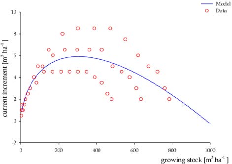
Such application of Richards function - first derivative - results, generally, in a high coefficient of determination (Fig. 1), that largely decrease with the increase of the number of quality classes forming the yield table (Fig. 2).
Fig. 1 - Example of Richards function (first derivative) fitting - Larix decidua. Comune di Cesana Torinese (TO) - Piano d’assestamento 1963-1972. Parameters: a = 446.1937; k = 0.0336; ν = 0.4889; y0= 0.21719; R2 = 0.9149003; ME= 0.9157618.
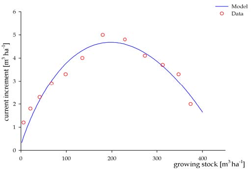
Fig. 2 - Example of Richards function (first derivative) fitting - Picea excelsa. Comune di Borno (BS). (Parameters: a = 978.6552; k = 0.0139; ν = -0.2757; y0= 0.06267; R2=0.54880459; ME= -2.794501).
Model structure
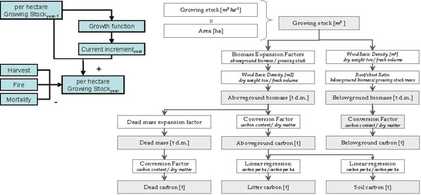
Using growing stock as unique driver, the model is able to estimate evolution in time of the five forest carbon pools, classified and defined according to Good Practice Guidance for LULUCF ([17]): aboveground and belowground biomass (living biomass), dead wood and litter (dead organic matter) and soil (soil organic matter - Fig. 3).
Fig. 3 - Model flowchart.
The methodology for growing stocks assessment in the years following NFI year is described as following:
- starting from initial growing stock volume (e.g., growing stock volume reported in the First Italian National Forest Inventory - [27]), for each year, the current increment per hectare [m3 ha-1 y-1] is computed with the derivative Richards function, for every specific forest typology;
- for each year, growing stock per hectare [m3 ha-1] is computed from the previous year growing stock volume adding the calculated current increment (“y” value of the derivative Richards) and subtracting losses due to harvest, mortality and fire occurred in the current year.
The process can be summarized as follows (eqn. 4):
in which current increment is calculated year by year by applying the derivative Richards function; and gsi is the volume per hectare of growing stock for current year; gsi-1 is the total previous year growing stock volume; Ii is calculated as f(vi-1) ·Ai-1 and is the total current increment of growing stock for current year; f is the Richards function reported above; νi-1 is the previous year growing stock volume per hectare; Ai-1 is the total area referred to a specific forest typology for previous year; Hi is the total amount of harvested growing stock for current year; Fi is the total amount of burned growing stock for current year; Mi is the total amount of growing stock removed by natural mortality; Di is the total amount of growing stock removed by drain and grazing (only in the category: protective forest).
Carbon amount released by forest fires has been included in the overall assessment of carbon stocks change. Since data on the fraction of growing stock oxidised as consequence of fires were not available, the most conservative hypothesis has been adopted; all growing stock of burned forest areas has been assumed to be completely oxidised and so released. Moreover, since data on forest typologies of burned areas were also not available, the total value of burned forest area coming from national statistics has been subdivided and assigned to forest typologies based on their respective weight on total national forest area. Finally, the amount of burned growing stock has been calculated multiplying average growing stock per hectare of forest typology for the assigned burned area. Assessed value has been subtracted to total growing stock of respective typology, as afore said.
Once estimated growing stock, amounts of aboveground woody tree biomass, belowground biomass and dead mass are consequently assessed.
Aboveground biomass
For every forest typology, starting from growing stock data, the amount of aboveground woody tree biomass (d.m.) [t] is estimated, for every forest typology, through the relation (eqn. 5):
where GS is the volume of growing stock [m3 ha-1]; BEF is the biomass expansion factor, which expands growing stock volume to volume of aboveground woody biomass; WBD is the wood basic density [t d.m. m-3 f.v.]; and A is the forest area occupied by a specific typology [ha].
Belowground biomass
For every forest typology, applying a Biomass Expansion Factor to growing stock data, the belowground biomass is estimated, with the following relation (eqn. 6):
where GS is the volume of growing stock [m3 ha-1]; R is the root/shoot ratio, which converts growing stock biomass in belowground biomass; WBD is the wood basic density [t d.m. m-3 f.v.]; A is the forest area occupied by a specific typology [ha].
Dead mass
For every forest typology, the deadwood mass was assessed applying a dead mass conversion factor (DCF, in accordance with Tab. 3.2.2 of GPG for LULUCF - [17]). The dead mass [t] is (eqn. 7):
where GS is the volume of growing stock [m3 ha-1]; BEF is the Biomass Expansion Factor which expands growing stock volume to volume of aboveground woody biomass; WBD is the Wood Basic Density [t d.m. m-3 f.v.]; DCF is the Dead mass Conversion Factor, which converts aboveground woody biomass in dead mass; A is the forest area occupied by a specific typology.
Litter
Total litter carbon amount is estimated from the carbon amount of aboveground biomass with linear relations. Linear relations between stand biomass and litter have been reported in many forest studies ([36]).
Soil
Applying linear relations, total soil carbon amount is estimated from carbon amount in aboveground biomass, following the same rationale as for litter carbon.
The carbon stocks change of living biomass (LB) is calculated according to Good Practice Guidance for LULUCF ([17]), from aboveground (AG) and belowground (BG) biomass (eqn. 8):
where total amount of carbon has been obtained from biomass (d.m.), multiplying by the GPG default factor for carbon fraction equal to 0.5.
The Dead Organic Matter (DOM) carbon pool is defined, in the GPG, as the sum of dead wood (D) and litter (L - eqn. 9):
The total amount of carbon for dead mass has been obtained from dead mass (d.m.), multiplying by the GPG default factor for carbon fraction equal to 0.5.
The Italian dataset
The above-described model has been applied to the Italian dataset, to assess carbon stocks in the five forest pools for reporting year 2007 of the Italian GHG’s Inventory.
The model has been applied at regional scale (NUT2) because of availability of any forest-related statistical data. Starting year of the model has been 1985 and estimates have been provided from 1986 to 2006.
Inventory typologies are classified in 4 main categories: Stands, Coppices, Plantations and Protective Forests: (i) Stands: norway spruce, silver fir, larches, mountain pines, mediterranean pines, other conifers, european beech, turkey oak, other oaks, other broadleaves. (ii) Coppices: european beech, sweet chestnut, hornbeams, other oaks, turkey oak, evergreen oaks, other broadleaves, conifers. (iii) Plantations: eucalyptuses coppices, other broadleaves coppices, poplar stands, other broadleaves stands, conifers stands, others. (iv) Protective Forests: rupicolous forest, riparian forests, shrublands.
Model input data for forest area, detailed by region and by forest typologies, come from the First Italian National Forest Inventory ([27]) and from the Second Italian National Forest Inventory. Forest area estimation for 1990 has been done through a linear interpolation between the 1985 and 2002 data (pers. comm., [18]). By assuming that defined trend may well represent near future, it was possible to extrapolate data for 2006.
For each of the five carbon pools, dataset and factors are set as explained in the following sections.
Woody aboveground biomass
Model input data of growing stocks for the start year (1985), detailed by region and by forest typologies come from the First Italian National Forest Inventory.
The average rate of mortality used for calculation have been 0.0116, concerning evergreen forests, and 0.0117, for deciduous forests, according to GPG for LULUCF ([17]).
The rate of draining and grazing, applied to protective forest, has been set as 3% following a personal judgement because total absence of referable data.
Total commercial harvested wood, for construction and energy purposes, has been obtained from national statistics ([19]); even if data on biomass removed in commercial harvest published by ISTAT are probably underestimated, particularly concerning fuelwood consumption ([1]). Data of wood use for construction and energy purposes, reported in m3, are disaggregated at NUT2 level, in sectoral statistics ([19], [20], [21]) or at NUT1 level for coppices and high forests in national statistics. These figures have been subtracted, as losses, to growing stock volume, as mentioned above.
Biomass Expansion Factors for conversions from growing stock volume to volume of aboveground biomass have been derived for each forest typology, using preliminary results of the RiselvItalia Project carried out by ISAFA ([18]), as follows:
- for broadleaves and pines with large crown: starting from stump, volume of whole woody biomass over bark up to 3 cm of diameter of all trees with diameter at breast height ≥ 3 cm;
- for conifers: starting from stump, wood volume of stem over bark up to 3 cm of diameter of all trees with diameter at breast height ≥ 3 cm.
Wood Basic Densities for conversions from fresh volume to dry weight have been derived for each forest typology, from [15]. In Tab. 2 BEF’s and WBD’s are reported.
Tab. 2 - Biomass Expansion Factors, Wood Basic Densities for aboveground biomass estimate and Root/Shoot ratio.
| Typology | Inventory typology |
BEF | Wood Basic Density |
R |
|---|---|---|---|---|
| volume of aboveground biomass / volume of growing stock | Dry weight t/ fresh volume of aboveground biomass m3 | weight of belowground biomass / weight of growing stock | ||
| Stands | norway spruce | 1.29 | 0.38 | 0.29 |
| silver fir | 1.34 | 0.38 | 0.28 | |
| larches | 1.22 | 0.56 | 0.29 | |
| mountain pines | 1.33 | 0.47 | 0.36 | |
| mediterranean pines | 1.53 | 0.53 | 0.33 | |
| other conifers | 1.37 | 0.43 | 0.29 | |
| european beech | 1.36 | 0.61 | 0.20 | |
| turkey oak | 1.45 | 0.69 | 0.24 | |
| other oaks | 1.42 | 0.67 | 0.20 | |
| other broadleaves | 1.47 | 0.53 | 0.24 | |
| partial total | 1.35 | 0.51 | 0.28 | |
| Coppices | european beech | 1.36 | 0.61 | 0.20 |
| sweet chestnut | 1.33 | 0.49 | 0.28 | |
| hornbeams | 1.28 | 0.66 | 0.26 | |
| other oaks | 1.39 | 0.65 | 0.20 | |
| turkey oak | 1.23 | 0.69 | 0.24 | |
| evergreen oaks | 1.45 | 0.72 | 1.00 | |
| other broadleaves | 1.53 | 0.53 | 0.24 | |
| conifers | 1.38 | 0.43 | 0.29 | |
| partial total | 1.39 | 0.56 | 0.27 | |
| Plantations | eucalyptuses coppices | 1.33 | 0.54 | 0.43 |
| other broadleaves coppices | 1.45 | 0.53 | 0.24 | |
| poplars stands | 1.24 | 0.29 | 0.21 | |
| other broadleaves stands | 1.53 | 0.53 | 0.24 | |
| conifers stands | 1.41 | 0.43 | 0.29 | |
| others | 1.46 | 0.48 | 0.28 | |
| partial total | 1.36 | 0.40 | 0.25 | |
| Protective | rupicolous forest | 1.44 | 0.52 | 0.42 |
| riparian forest | 1.39 | 0.41 | 0.23 | |
| shrublands | 1.49 | 0.63 | 0.62 | |
| partial total | 1.46 | 0.56 | 0.50 | |
| Total | - | 1.38 | 0.53 | 0.30 |
Belowground biomass
Also in this case, the values for root/shoot ratio Rs, reported in Tab. 2, were derived for each forest typology, in the same way as for aboveground biomass. Values refer to all living biomass of live roots; fine roots of less than (suggested) 2 mm diameter are often excluded because these often cannot be distinguished empirically from soil organic matter or litter.
Dead mass
The deadwood mass was assessed applying a dead mass conversion factor (DCF of respectively 0.2 for evergreen forests and 0.14 for deciduous forests, as reported in Tab. 3.2.2 of GPG - [17]).
Tab. 3 - Relations: litter and soil carbon - aboveground carbon per ha.
| Category | Inventory typology | Relation litter Aboveground C / ha |
Relation soil Aboveground C / ha |
|---|---|---|---|
| Stands | norway spruce | y = 0.0659x + 1.5045 | y = 0.4041x + 57.874 |
| silver fir | y = 0.0659x + 1.5045 | y = 0.4041x + 57.874 | |
| larches | y = 0.0659x + 1.5045 | y = 0.4041x + 57.874 | |
| mountain pines | y = 0.0659x + 1.5045 | y = 0.4041x + 57.874 | |
| mediterranean pines | y = 0.0659x + 1.5045 | y = 0.4041x + 57.874 | |
| other conifers | y = 0.0659x + 1.5045 | y = 0.4041x + 57.874 | |
| european beech | y = -0.0299x + 9.3665 | y = 0.9843x + 5.0746 | |
| turkey oak | y = -0.0299x + 9.3665 | y = 0.9843x + 5.0746 | |
| other oaks | y = -0.0299x + 9.3665 | y = 0.9843x + 5.0746 | |
| other broadleaves | y = -0.0299x + 9.3665 | y = 0.9843x + 5.0746 | |
| Coppices | european beech | y = -0.0299x + 9.3665 | y = 0.3922x + 65.356 |
| sweet chestnut | y = -0.0299x + 9.3665 | y = 0.3922x + 65.356 | |
| horbeams | y = -0.0299x + 9.3665 | y = 0.3922x + 65.356 | |
| other oaks | y = -0.0299x + 9.3665 | y = 0.3922x + 65.356 | |
| turkey oak | y = -0.0299x + 9.3665 | y = 0.3922x + 65.356 | |
| evergreen oaks | y = -0.0299x + 9.3665 | y = 0.3922x + 65.356 | |
| other broadleaves | y = -0.0299x + 9.3665 | y = 0.3922x + 65.356 | |
| conifers | y = 0.0659x + 1.5045 | y = 0.4041x + 57.874 | |
| Plantations | eucalyptuses coppices | y = -0.0299x + 9.3665 | y = 0.3922x + 65.356 |
| other broadleaves coppices | y = -0.0299x + 9.3665 | y = 0.3922x + 65.356 | |
| poplars stands | y = -0.0299x + 9.3665 | y = 0.9843x + 5.0746 | |
| other broadleaves stands | y = -0.0299x + 9.3665 | y = 0.9843x + 5.0746 | |
| conifers stands | y = 0.0659x + 1.5045 | y = 0.4041x + 57.874 | |
| others | y = -0.0165x + 7.3285 | y = 0.7647x + 33.638 | |
| Protective | rupicolous forest | y = -0.0165x + 7.3285 | y = 0.7647x + 33.638 |
| riparian forest | y = -0.0299x + 9.3665 | y = 0.9843x + 5.0746 | |
| shrublands | y = -0.0299x + 9.3665 | y = 0.3922x + 65.356 |
Litter
It includes all non-living biomass with a diameter less than a minimum diameter chosen by the country for lying dead (for example 10 cm), in various states of decomposition above the mineral or organic soil. This includes the litter, fumic, and humic layers. Live fine roots (of less than the suggested diameter limit for below-ground biomass) are included in litter where they cannot be distinguished from it empirically.
Up to now we do not have a full comprehensive data set to establish a more proper biophysical relation for Italian forests. But collection of data in the Italian new national forest inventory should allow to analyze the relationship and to choose most appropriate mathematical representation. For present work we have used the results of the European project CANIF (⇒ http://www.bgc-jena.mpg.de/bgc-processes/research/Schulze_Euro_CANIF.html#contents) which has reported such relations for a number of European forest stands. The total litter carbon amount has been estimated from aboveground carbon amount with linear relations differentiated per forestry use: stands (resinous, broadleaves, mixed stands) and coppices (Tab. 3).
Soil
To this purpose we have used data coming from a number of permanent plots, distributed in several forest typologies, within the project CONECOFOR (⇒ http://www.corpoforestale.it/wai/serviziattivita/CONECOFOR/index.htm) of the Italian Ministry of Agriculture and Forestry, which provided data on stand biomass and soil carbon. Per forestry use: stands (resinous, broadleaves, mixed stands) and coppices, total soil carbon amount [t C ha-1] has been estimated from carbon amount of total woody aboveground biomass [t C ha-1], with linear relations. In Tab. 3 the used relations have been reported.
Results and discussion
In the reported case of study, the For-est model has been applied to Italian dataset, in order to provide estimates of carbon stocks changes in the five forest pools: aboveground, belowground and dead mass, soil and litter (Fig. 4). In the following tables (Tab. 4 and Tab. 5), carbon stocks in the above mentioned pools and carbon stock changes are shown.
Fig. 4 - Carbon stock in the five carbon pools [Gg CO2 equivalent].
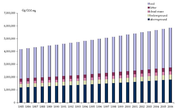
Tab. 4 - Carbon stocks in the five carbon pools [Gg CO2 equivalent].
| Year | living biomass | dead organic matter | soil organic matter |
total | ||
|---|---|---|---|---|---|---|
| aboveground | belowground | dead mass | litter | Soil | ||
| 1985 | 1195445 | 273629 | 180432 | 237858 | 2296283 | 4183646 |
| 1986 | 1219454 | 278155 | 183507 | 240877 | 2331502 | 4253495 |
| 1987 | 1241906 | 282299 | 186357 | 243926 | 2365635 | 4320122 |
| 1988 | 1263786 | 286372 | 189130 | 247061 | 2399733 | 4386082 |
| 1989 | 1288949 | 291217 | 192312 | 250061 | 2435865 | 4458404 |
| 1990 | 1307136 | 294627 | 194425 | 253141 | 2468297 | 4517626 |
| 1991 | 1336836 | 300486 | 198270 | 256090 | 2506809 | 4598490 |
| 1992 | 1364584 | 305907 | 201852 | 259086 | 2544270 | 4675700 |
| 1993 | 1385098 | 309730 | 204595 | 262246 | 2576800 | 4738468 |
| 1994 | 1414023 | 315450 | 208465 | 265223 | 2614371 | 4817532 |
| 1995 | 1445453 | 321838 | 212575 | 268160 | 2653922 | 4901947 |
| 1996 | 1478567 | 328579 | 217010 | 271103 | 2694039 | 4989297 |
| 1997 | 1507848 | 334508 | 220890 | 274093 | 2731941 | 5069279 |
| 1998 | 1536363 | 340190 | 224707 | 277042 | 2768860 | 5147161 |
| 1999 | 1568504 | 346799 | 229142 | 280018 | 2808277 | 5232741 |
| 2000 | 1597791 | 352703 | 233178 | 283057 | 2845515 | 5312244 |
| 2001 | 1631400 | 359586 | 237801 | 286044 | 2885499 | 5400330 |
| 2002 | 1668344 | 367203 | 242900 | 288986 | 2927452 | 5494885 |
| 2003 | 1700073 | 373692 | 247282 | 291995 | 2966507 | 5579550 |
| 2004 | 1735805 | 381056 | 252229 | 294992 | 3008005 | 5672088 |
| 2005 | 1771367 | 388414 | 257127 | 297971 | 3049532 | 5764411 |
| 2006 | 1803549 | 395100 | 261601 | 300992 | 3088758 | 5850001 |
Tab. 5 - Carbon stock changes in the five carbon pools [Gg CO2 equivalent].
| Year | living biomass | dead organic matter | soil organic matter |
total | ||
|---|---|---|---|---|---|---|
| aboveground | belowground | dead mass | litter | soil | ||
| 1986 | 24009 | 4526 | 3076 | 3019 | 35219 | 69848 |
| 1987 | 22452 | 4145 | 2849 | 3049 | 34133 | 66627 |
| 1988 | 21881 | 4073 | 2773 | 3135 | 34098 | 65960 |
| 1989 | 25163 | 4844 | 3183 | 3001 | 36132 | 72322 |
| 1990 | 18187 | 3410 | 2113 | 3079 | 32432 | 59222 |
| 1991 | 29700 | 5859 | 3845 | 2949 | 38512 | 80864 |
| 1992 | 27748 | 5422 | 3582 | 2996 | 37462 | 77209 |
| 1993 | 20514 | 3822 | 2743 | 3159 | 32529 | 62768 |
| 1994 | 28925 | 5721 | 3870 | 2977 | 37572 | 79064 |
| 1995 | 31430 | 6388 | 4110 | 2937 | 39550 | 84415 |
| 1996 | 33114 | 6742 | 4435 | 2943 | 40117 | 87350 |
| 1997 | 29281 | 5928 | 3880 | 2991 | 37902 | 79982 |
| 1998 | 28515 | 5682 | 3817 | 2949 | 36919 | 77882 |
| 1999 | 32141 | 6610 | 4436 | 2976 | 39417 | 85580 |
| 2000 | 29287 | 5903 | 4036 | 3039 | 37238 | 79503 |
| 2001 | 33609 | 6883 | 4623 | 2986 | 39984 | 88086 |
| 2002 | 36945 | 7617 | 5099 | 2942 | 41952 | 94555 |
| 2003 | 31729 | 6489 | 4383 | 3010 | 39055 | 84665 |
| 2004 | 35732 | 7364 | 4947 | 2996 | 41498 | 92538 |
| 2005 | 35562 | 7358 | 4897 | 2979 | 41526 | 92323 |
| 2006 | 32182 | 6686 | 4474 | 3021 | 39227 | 85590 |
It can be noted that in 2006 the Italian total carbon stock in forest sector amounts to about 5.8 Gt CO2 with the largest pool constituted by soil carbon. The ratio of aboveground biomass to soil carbon is about 0.58 which is higher than the one (circa 45%) calculated for other European countries from the data reported in the FAO - Global Forest Resources Assessment ([14]). The three other pools (below ground, dead wood and litter) are almost equivalent and amount to about 7%, 4% and 5% of total, respectively.
The increasing trend of the five pools reflects in this case the expansion of forest areas which occurred in the period 1986 - 2006.
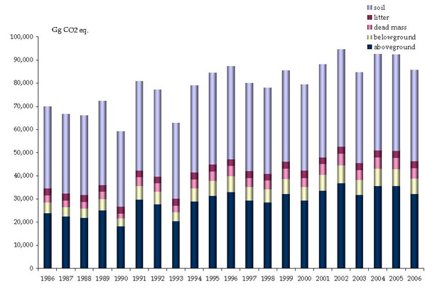
By contrast stock changes in aboveground biomass are comparable with changes in soil carbon stocks (Fig. 5). The values showed in Tab. 5, if reported at the stand level shows an average 1986-2006 accumulation rate of 7.94 t CO2 ha-1 y-1 (living biomass 3.47 t CO2 ha-1 y-1; dead organic matter: 0.69 t CO2 ha-1 y-1; soil: 3.79 t CO2 ha-1 y-1). In general, this result seems to show some overestimation of soil carbon changes, and it is due also to the fact that when new forest area is added then, automatically, the whole soil carbon stock of such area is added to the total resulting in an increase of total carbon stock that is actually no more than a shifting of stocks from one land use category (i.e., grassland) to another (i.e., forest land).
Fig. 5 - Carbon stock changes in the five carbon pools [Gg CO2 equivalent].
Tab. 6 shows values of current increment reported on National Forest Inventory ([27]) for different forest typologies. In the same table, the values of current increment assessed by Richards functions are also reported, calibrated on yield tables data. Comparison between measured and estimated values is only feasible for high stands, since only for this silvicultural system the values of current increments are reported in the first NFI.
Tab. 6 - NFI’s and estimated current increment values for different forest typologies (stands).
| Forest typology | current increment reported in the 1st NFI (1985) | current increment estimated with Richards functions |
|---|---|---|
| high stands | m3 ha-1 | m3 ha-1 |
| norway spruce | 9.4 | 5.7 |
| silver fir | 9.2 | 7.0 |
| larches | 5.7 | 4.4 |
| mountain pines | 8 | 8.5 |
| mediterranean pines | 7.1 | 8.7 |
| other conifers | 13.6 | 6.5 |
| european beech | 8.5 | 7.0 |
| turkey oak | 6.7 | 5.2 |
| other oaks | 4.6 | 4.3 |
| other broadleaves | 8.8 | 5.2 |
| average | 7.9 | 6.3 |
In Fig. 6, current increments estimated with the Richards function are plotted against current increment data obtained by the first Italian NFI. Because wide majority of the points are in the lower half of Cartesian field, it is possible to state that the model shows a systematic underestimation of current increments (in particular the estimated average value is 20% smaller).
Fig. 6 - Current increment reported on NFI vs current increment estimated with Richards.
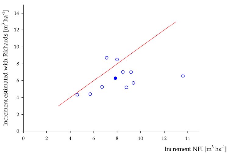
The mismatch between the estimated and reported NFI data is likely to be caused by a general disagreement between yield tables and the real average quality of forest sites in the country. The Richards function was parametrised using all yield tables quality classes, on average, without weighting different contributes of different classes.
Moreover, the available yield tables are somewhat outdated since they were compiled mainly during the years 1950-1970. Nowadays a higher current increment than in the past is most likely, as confirmed in other countries like Germany (see ⇒ http://www.bundeswaldinventur.de) due to increased temperatures, atmospheric CO2 concentration and nitrogen deposition ([28]), as well as changes in forest management, based also on the conclusion of the IPCC expert meeting on current scientific understanding of the processes affecting terrestrial carbon stocks and human influences upon them (Geneva, Switzerland 21-23 July 2003).
Beside to the possible underestimate of current increment, it should be noted that losses by harvested wood are underestimated too, particularly concerning fuelwood consumption. In the estimation process of growing stock time series, a sort of compensation is very likely to occur between underestimated current increment and underestimated harvesting.
Further improvements in refining current increment estimate will be possible when more basic data and information from the second national forest inventory will be available.
Uncertainty
To assess overall uncertainty related to estimates for years 1990-2006, we followed the GPG Tier 1 Approach. The uncertainty linked to the year 1985, when first National Forest Inventory was carried out, was calculated with the relation (eqn. 10):
where overall uncertainty E is expressed by the terms Vi indicating each of the carbon stocks of the five pools for the year 1985 (i = AG: aboveground, BG: belowground, D: dead mass, L: litter, S: soil), while, with letter E, related uncertainties have been indicated. Tab. 7 shows the equations for assessing the overall uncertainties associated to the carbon pools.
Tab. 7 - Relations for assessing uncertainties of C pools.
| Carbon pool | Relation for uncertainty assessing |
|---|---|
| Aboveground | EAB_1985 = (ENFN2 + EBEF2 + EBD2 + ECF2)0.5 |
| Belowground | EBG_1985 = (ENFI2 + ER2 + EBD2 + ECF2)0.5 |
| Dead mass | ED_1985 = (EAG_19852 + EDCF_19852)0.5 |
| Litter | EL_1985 = (ELS_19852 + ELR_s2)0.5 |
| Soil | ES_1985 = (ESS_19852 + ESR_s2)0.5 |
Terminology for aboveground: ENFI = uncertainty associated to growing stock data given by the first National Forest Inventory; EBF = uncertainty related to biomass expansion factors for aboveground biomass; EBD = uncertainty of the basic density; ECF = uncertainty of the conversion factor, where GPG default values for uncertainty assessment have been used ([17]).
Terminology for belowground: ER = uncertainty of root-shoot-ratio taken from GPG default. Concerning dead mass relation, EDCF = uncertainty of dead mass expansion factor, taken from GPG default; ELS_1985 and ESS_1985 = uncertainties related to litter and soil carbon stock data taken from CANIF project and CONECOFOR Programme, respectively. Finally, the terms ELR_1985 and ESR_1985 are defined as uncertainties related to linear regressions used to assessing litter and soil carbon stocks. Tab. 8 shows the values of carbon stocks in the five pools for year 1985, with the associated uncertainties.
Tab. 8 - Carbon stocks and uncertainties for year 1985 and current increment related uncertainty. (a) The current increment is estimated by the Richards function (first derivative); uncertainty has been assessed considering the standard error of the linear regression between the estimated values and the corresponding current increment values reported in the National Forest Inventory. (b) Good Practice Guidance default value ([17]).
| Carbon stocks t and CO2 eq. ha-1 | Aboveground biomass | VAG 137.8 |
| Belowground biomass | VBG 31.5 | |
| Dead mass | VD 20.8 | |
| Litter | VL 27.4 | |
| Soil | VS 264.7 | |
| Uncertainty | Growing stock | ENFI 3.2% |
| Current increment (Richards)(a) | ENFI 51.6% | |
| Harvest(b) | EH 30% | |
| Fire(b) | EF 30% | |
| Drain and grazing | ED 30% | |
| Mortality | EM 30% | |
| BEF | EBEF1 30% | |
| R | EBEF2 30% | |
| DCF | EDEF 30% | |
| Litter (stock + regression) | EL 161% | |
| Soil (stock + regression) | ES 152% | |
| Basic Density | EBD 30% | |
| C Conversion Factor | ECF 2% |
Tab. 9 shows the uncertainties related to individual carbon pools and the overall uncertainty for 1985, as based on the equations in Tab. 7.
Tab. 9 - Uncertainties related to carbon pools and overall uncertainty for year 1985.
| Aboveground biomass | EAG 42.59% |
| Belowground biomass | EBG 42.59% |
| Dead mass | ED 52.10% |
| Litter | EL 161.22% |
| Soil | ES 152.05% |
| Overall uncertainty | E1985 84.91% |
The overall uncertainty related to 1985 (year of the first National Forest Inventory) was propagated until 2006, following the Tier 1 approach.
The equations for the year following to 1985 are similar to the one for the 1985 uncertainty estimate, apart from terms linked to aboveground biomass: the biomass increment was computed by the methodology described in Model structure paragraph; in consequence, the related uncertainty, e.g., for 1986, is expressed by the following formula (eqn. 11):
where i = NFI, I, H, F, D, M.
Following Tier 1 approach and the above mentioned methodology, the overall uncertainty in the estimates produced by the described model has been quantified; in Tab. 10 the uncertainties of the 1985-2006 period are reported.
Tab. 10 - Overall uncertainties 1985 - 2006.
| Year | Perc. |
|---|---|
| 1985 | 84.91% |
| 1986 | 84.81% |
| 1987 | 88.09% |
| 1988 | 88.32% |
| 1989 | 88.26% |
| 1990 | 88.25% |
| 1991 | 88.15% |
| 1992 | 87.97% |
| 1993 | 87.93% |
| 1994 | 87.84% |
| 1995 | 87.65% |
| 1996 | 87.46% |
| 1997 | 87.32% |
| 1998 | 87.22% |
| 1999 | 87.07% |
| 2000 | 86.93% |
| 2001 | 86.77% |
| 2002 | 86.57% |
| 2003 | 86.41% |
| 2004 | 86.27% |
| 2005 | 86.09% |
| 2006 | 85.97% |
The overall uncertainty in the model estimates between 1985 and 2006 was assessed with the following relation (eqn. 12):
where terms V1985 and V2006 represent growing stocks in [m3 ha-1 CO2 eq], E the uncertainties in the respective years. The overall uncertainty related to the period 1985-2006 is equal to 60.5%.
However, on May 29th 2007, during a national workshop on forest statistics, the preliminary data of the new NFI regarding to the 2006 aboveground carbon stock of the whole Italian forest land area were presented. A comparison between our estimate and the preliminary NFI data results in 1.2% difference (Tab. 11).
Tab. 11 - Comparison between modelized and NFI preliminary 2006 aboveground carbon stock.
| NFI aboveground carbon stock (tC) |
For-est model related to 2006 (tC) |
|---|---|
| 486018500 | 491877087 |
Conclusions
The proposed approach has provided both a reanalysis of the Italian forest sector carbon stock changes in accordance with UNFCCC requirements and estimates of carbon stock changes for years between national forest inventories.
The use of an age-independent relationship for deriving forest growth increment, from growing stocks has been proven more useful than a classical age-growth relationship.
In particular, the approach allows deriving from the growing stock the other carbon budget components, which are usually difficult to obtain, or for which detailed process based models are still far from being operational. Using a single input like growing stock, which is regularly derived from NFI, is particularly useful: it is directly assessed and can more easily be verified by different methodologies like verification plots or remote sensing techniques.
Based on our novel approach, using NFI data of 1985 and including the new forest areas estimates of 2004 (pers. comm., MAF-ISAFA 2004), we calculate an overall carbon stock change for Italian forest in 2006 in the range 85 Mt CO2. This estimate is rather conservative since the approach based on an overall Richard function approximation tends to underestimate the observed increment by NFI.
Improvements of the above mentioned approach could be driven by the web-based “AFOLU-Clearinghouse for Policy-Science-Data” under development by JRC, especially with regard to its European level databases of allometric biomass & carbon factors, yield tables and forest inventories (see ⇒ http://afoludata.jrc.it/carboinvent/ciintro.cfm). The approach described above in combination with such database will improve quality control and quality assurance routines (e.g., verification, cross-checking) for national GHG inventories and will help in gap-filling of the forestry sector in the EC-Inventory.
Finally, it is worth to note that data produced by this methodology have been successfully used by the Italian government for the renegotiation of the Italian cap for the forest management activity under Article 3.4 of the Kyoto Protocol (FCCC/KP/CMP/2006/10/Add.1 - Decision 8/CMP.2, Forest management under Article 3, paragraph 4, of the Kyoto Protocol: Italy). A fundamental step in the renegotiation process has been the peer review of data and methodologies by the UNFCCC experts, resulting in no major findings.
The Italian cap passes from 0.18 Mt C to 2.78 Mt C, with a strong impact on the economic value associated to the Italian forest, being an incentive in the conservation and sustainable management of the forest areas.
References
Gscholar
Gscholar
Gscholar
Gscholar
Gscholar
Gscholar
Gscholar
Gscholar
Gscholar
Gscholar
Gscholar
Gscholar
Gscholar
CrossRef | Gscholar
Gscholar
Gscholar
Authors’ Info
Authors’ Affiliation
S Tulipano
G Seufert
European Commission’s Joint Research Centre, Climate Change Unit, v. E. Fermi 1, Ispra, Varese (Italy)
R De Lauretis
APAT, Agenzia per la Protezione dell’Ambiente e per i Servizi Tecnici, v. C. Pavese 313, Roma (Italy)
Corresponding author
Paper Info
Citation
Federici S, Vitullo M, Tulipano S, De Lauretis R, Seufert G (2008). An approach to estimate carbon stocks change in forest carbon pools under the UNFCCC: the Italian case. iForest 1: 86-95. - doi: 10.3832/ifor0457-0010086
Paper history
Received: Jun 14, 2007
Accepted: Jan 24, 2008
First online: May 20, 2008
Publication Date: May 20, 2008
Publication Time: 3.90 months
Copyright Information
© SISEF - The Italian Society of Silviculture and Forest Ecology 2008
Open Access
This article is distributed under the terms of the Creative Commons Attribution-Non Commercial 4.0 International (https://creativecommons.org/licenses/by-nc/4.0/), which permits unrestricted use, distribution, and reproduction in any medium, provided you give appropriate credit to the original author(s) and the source, provide a link to the Creative Commons license, and indicate if changes were made.

Web Metrics
Breakdown by View Type
Article Usage
Total Article Views: 61589
(from publication date up to now)
Breakdown by View Type
HTML Page Views: 46041
Abstract Page Views: 6472
PDF Downloads: 7737
Citation/Reference Downloads: 92
XML Downloads: 1247
Web Metrics
Days since publication: 6642
Overall contacts: 61589
Avg. contacts per week: 64.91
Article Citations
Article citations are based on data periodically collected from the Clarivate Web of Science web site
(last update: Mar 2025)
Total number of cites (since 2008): 68
Average cites per year: 3.78
Publication Metrics
by Dimensions ©
Articles citing this article
List of the papers citing this article based on CrossRef Cited-by.
Related Contents
iForest Similar Articles
Research Articles
Assessing the carbon sink of afforestation with the Carbon Budget Model at the country level: an example for Italy
vol. 8, pp. 410-421 (online: 02 October 2014)
Technical Reports
Allometric biomass and carbon factors database
vol. 1, pp. 107-113 (online: 09 July 2008)
Research Articles
Estimating carbon dynamics in forest carbon pools under IPCC standards in South Korea using CBM-CFS3
vol. 10, pp. 83-92 (online: 13 October 2016)
Research Articles
Carbon stock in Kolli forests, Eastern Ghats (India) with emphasis on aboveground biomass, litter, woody debris and soils
vol. 4, pp. 61-65 (online: 05 April 2011)
Research Articles
Effects of tree species, stand age and land-use change on soil carbon and nitrogen stock rates in northwestern Turkey
vol. 9, pp. 165-170 (online: 18 June 2015)
Commentaries & Perspectives
What happened to forests in Copenhagen?
vol. 3, pp. 30-32 (online: 02 March 2010)
Research Articles
Do the rubber plantations in tropical China act as large carbon sinks?
vol. 7, pp. 42-47 (online: 21 October 2013)
Research Articles
Spatially explicit estimation of forest age by integrating remotely sensed data and inverse yield modeling techniques
vol. 9, pp. 63-71 (online: 25 July 2015)
Research Articles
Patterns of carbon allocation in a chronosequence of Caragana intermedia plantations in the Qinghai-Tibet Plateau
vol. 8, pp. 756-764 (online: 08 April 2015)
Research Articles
Soil C:N stoichiometry controls carbon sink partitioning between above-ground tree biomass and soil organic matter in high fertility forests
vol. 8, pp. 195-206 (online: 26 August 2014)
iForest Database Search
Search By Author
Search By Keyword
Google Scholar Search
Citing Articles
Search By Author
Search By Keywords
PubMed Search
Search By Author
Search By Keyword


