Making objective forest stand maps of mixed managed forest with spatial interpolation and multi-criteria decision analysis
iForest - Biogeosciences and Forestry, Volume 6, Issue 5, Pages 268-277 (2013)
doi: https://doi.org/10.3832/ifor0099-006
Published: Jul 01, 2013 - Copyright © 2013 SISEF
Research Articles
Abstract
The spatial interpolation and multi-criteria decision analysis (MCDA) capabilities of geographic information systems have the potential to create new approaches to forest management. In this study of heterogeneously structured stand maps, the potential use of the regularized spline with tension (RST) interpolation method and of ELECTRE TRI MCDA was investigated. For each species and diameter class, one map of the predicted volume per ha was produced with the RST method. The map used data from a total of 1050 circular sample plots. By repeating the same process for the eight species occurring in the study area, 31 volume maps were produced. The accuracy of these prediction maps was calculated at the pixel (20 x 20 m) level and at the area level (per ha). An accuracy of greater than or equal to 97% was achieved at the pixel level, whereas a minimum accuracy of 86% was achieved for the area-based calculations. In addition, these 31 volume maps were compared with the management report results obtained from the government institute responsible for defining management plans. These comparisons were performed for the total volume of all species with volume ratios greater than 1%. The comparisons showed 21, 14, 4, and 2 % accuracies for Calabrian pine, Oriental beech, black pine and oak species, respectively. Following interpolation, these 31 maps were geo-computed, and a volume-based stand map was produced. The 890 different mixture variations resulting from combinations of the volume of species composition and the stand diameter class in these maps were classified according to expert knowledge. In this classification process, ELECTRE TRI MCDA was used to benefit from the capabilities provided by geographic information systems. Finally, ELECTRE TRI was used to reduce the 890 different mixture combinations to 70 stand type classes.
Keywords
Regularized Spline with Tension, Multi-Criteria Decision Analysis, Forest Map, Forest Management
Introduction
Information about extant forest communities is of considerable importance in forest management planning. The stand is the smallest production and silvicultural unit, and the most crucial part of this information. The location of planning units, their size and silvicultural features are used to select management objectives and determine the working cycle, management regulations and silvicultural goals. Thus, the precision of decisions to be implemented and the planning to be realized are both closely related to the accuracy of the stand maps. Moreover, map accuracy depends on the type of forest inventory, the sample size, and the techniques used to evaluate the inventory results.
Stand maps have previously been produced subjectively ([13]) in conjunction with current forest management practices. In conventional management planning, stands are defined through the planning process. The type of of the management objectives is a component of this process ([20]). However, the use of computers has changed this conventional approach, and spatially and temporally dynamic description and treatment units can readily be produced ([25]). Thus, dynamic forest planning can be achieved with the use of geopositioned field plot data and computers ([64]).
The sampling methods used in forest inventories vary according to different countries’ forestry objectives and forest structures. Systematic sampling methods are recommended for large and homogeneous forest areas and have been implemented in all production and conservation areas of Turkey since 1964. However, if this sampling method is implemented with an insufficient number of sample plots and/or in heterogeneous forests, the results will be highly questionable because they may fail to reflect the true forest composition. Although Sherman ([55]), Aurbi & Debouzie ([5]), Flores et al. ([14]) and D’Orazio ([10]) used remote sensing data to improve the results of such inventories, the desired outcome was never achieved in practice.
Spatial interpolation methods, which have been classified by Li & Heap ([37]) as non-geostatistical, geostatistical and combined, came into use at the end of the 1960s and have been investigated for use in forest management. As described in Akhavan et al. ([1]), Guibal ([19]) was the first study to use kriging in the forest inventory process. Jost ([28]) also used geostatistical methods to compare conventional inventory results based on systematic sampling with the results of the kriging method. Geostatistically based methods that utilize textural information are frequently used to analyze remote-sensing (RS) images ([66]). The quality and quantity of these methods have increased through advances in the computer sciences and in the science of geographical information systems. These methods allow the use of a variety of ecological and technical parameters in the assessment of inventory results.
Palmer et al. ([50]) compared the spatial predictions derived from Inverse Distance Weighting (IDW), Partial Least Squares (PLS), Regression Kriging (RK), and Ordinary Kriging (OK) for Pinus radiata mean volume, annual increment and mean top height. Viana et al. ([63]) made estimations of the crown biomass of Pinus pinaster stands and aboveground shrubland biomass using forest inventory data, remotely sensed imagery for auxiliary variables and spatial prediction models. These estimations involved the use of RK and OK, Universal Kriging (UK), IDW and Thiessen Polygon estimations. Magnussen et al. ([40]) examined the advantages of multiresolution spatial models (MRSMs) for large datasets compared with standard algorithms.
Montes et al. ([46]) have proposed a method in which the addition of experienced inventory data areas are combined with environmental information. Nanos et al. ([47]) also used a geostatistical approach for the prediction of diameter distributions in stands of Pinus pinaster Ait. Tang & Bian ([58]) successfully applied a forest site evaluation method which integrates a geographic information system (GIS) and a spatial interpolation method (kriging) in geostatistics.
Köhl et al. ([34]) suggested the use of aerial photographs, satellite images, site data, and thematic maps in the analysis and modeling of survey plans. Mandallaz ([41]) compared different geostatistical methods in forest inventory creation. Höck et al. ([27]) evaluated the kriging method using site index data. Holmgren & Thuresson ([25]) used kriging and remote sensing to predict stand volumes.
Heikkinen ([22]) and many other researchers reported that the determination of sampling errors was a serious problem associated with systematic sampling. To obtain greatly improved results from systematic sampling and inventory measurements, the use of additional explanatory environmental variables has been initiated ([36]).
Recently, the production of stand maps based on GIS has started to develop forest management planning in Turkey. Since 2004, computers have been used to perform stand type delineations and generalizations with classical and subjective operator-oriented methods and to produce digital maps of high cartographic quality. However, as emphasized by Burrough ([7]), the spatial and statistical analysis capabilities of GIS have not been fully explored and exploited yet. In contrast, GIS capabilities, combined with different spatial interpolation methods and multi-criteria decision analysis (MCDA), are being developed and implemented in numerous disciplines.
ELECTRE (ELimination Et Choix Traduisant la REalité - Elimination and Choice Expressing the Reality) is family of methods derived from MCDA that associate members to create an alternative set of relationships within the system, and then compare the alternatives obtained to solve the problem under investigation. The main advantage of these methods is that the optimal solution is not subjective, avoiding classical approaches based on individual experience and intuition. Diverse ELECTRE methods differ in minor respects. For instance, ELECTRE TRI was created to solve selection and assignment problems.
A review of more than 250 papers in the forestry literature over the past 30 years showed that 9 different versions of MCDA were applied to 9 different forestry topics (wood production, biodiversity, sustainability, reforestation, regional planning, forest industry, risks, and other subjects - [6]). A variant of the ELECTRE method was recommended by Kangas et al. ([30]) who discussed the application of the ELECTRE III and PROMETHEE II methods in 17 forest activity areas. Mendoza & Martins ([42]) critically reviewed the MCDA methods applied to the management of forests and other natural resources, describing the nature of these models and their inherent strengths and limitations. Jayanath & Gamini ([35]) also provided a comprehensive literature review in forest management evaluating 9 different types of MCDA in terms of their theoretical basis and the risks associated with their use. Currently, many opinions and suggestions exist regarding the use of MCDA in forestry. It has been claimed that MCDA alone may not be sufficient for use in forest management. On the other hand, hybrid approaches has been reported as suitable for application in this field ([29]).
Because each mapping expert has different knowledge and experience, traditional management plans can show spatial and temporal differences. To solve the above discrepancies, management plans produced using objective criteria and suitable methods (like GIS) may help to achieve consistency among maps pertaining to different revision periods and/or maps of adjacent planning units.
The main goal of this study is the creation of semi-automated, objective maps based on forest stand volume calculated from ground survey data. To achieve this goal, the spatial analysis capability of GIS was used. The regularized spline with tension (RST) spatial interpolation method was used to produce volume prediction maps of species, and ELECTRE TRI MCDA was applied to create the final forest map needed for objective decision making.
Materials and methods
Study Area
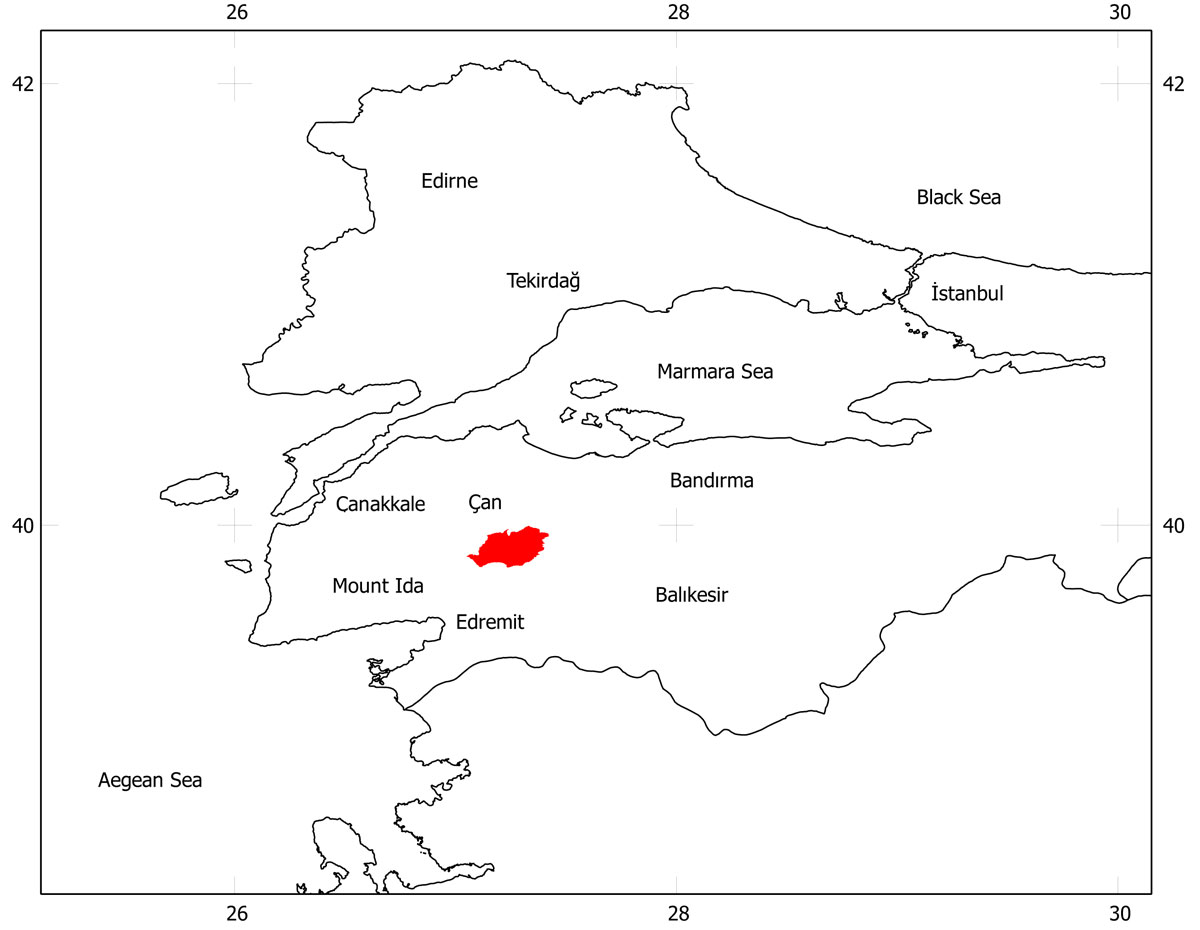
The study was conducted in the Asar and the Yenice forest ranges, two managed forest areas located on Mount Ida in Turkey (Fig. 1). The Asar range includes 11 159 ha of productive and 2473 ha of non-productive area. In the Yenice range the productive and non-productive areas are 10 817 ha and 1816 ha, respectively. The terrain is hilly throughout these forests. Minimum and maximum elevation are 100 m and 1.000 m a.s.l., respectively. The primary tree species found are oak species (Quercus sp.), Anatolian black pine (Pinus nigra Arn.), Calabrian pine (Pinus brutia Ten), Oriental beech (Fagus orientalis Lipsky), common hornbeam (Carpinus betulus L.), Trojan fir (Abies nordmanniana (Stev.) Spach. subsp. equi-trojani (Asch. & Sint. ex Boiss.) Coode & Cullen), Spanish chestnut (Castanea sativa Mill.) and other deciduous species (e.g., silver lime (Tilia sp.), Alnus glutinosa L. - [3], [4]).
Fig. 1 - The study area.
Total forest acreage for Turkey in 2004 was 21 188 747 ha (1 831 536 ha of deciduous forests, 11 403 791 ha of coniferous forests, 2 204 268 ha of mixed forests and 5 749 152 ha of coppice ([16]).
The study area is mainly covered by mixed forests, whose structural heterogeneity is known to hinder the application of interpolation methods, thus representing a challenging test for the assessment of the applied methodology in such environments.
Vegetation Data
The 2010 management year inventory data for the Asar and Yenice forest range were used in this study. The inventory data consisted of 1 050 circular sample plots (size: 200, 400, 600, and 800 m2) systematically placed at 300 m intervals. Within each plot, measurements were taken for diameter, mean height, top height, age, health status and stem quality of each tree. The most frequent sampling plot size was chosen to achieve a pixel resolution for the interpolation maps equal to the size of the sample plots of development age c (400 m2 - see below). Due to the inventory method adopted, the forest structure within approximately 50 m of the center of the sample plot was checked visually. Any distinctive, observable characteristics within the plot and along the path from plot to plot were recorded.
The classification of even-aged stands was performed according to the 2008 Turkish forest management instructions. Diameter ranges were grouped in the following classes: (a) 1.0-7.9 cm; (b) 8.0-19.9 cm; (c) 20.0-35.9 cm; (d) 36.0-51.9 cm; and (e) > 52.0 cm. In diameter class a, no measurements were taken for the calculation of stand parameters.
Forest inventory and the production of stand maps in Turkey include the following steps:
- The management-planning unit is divided into homogeneous segments based on remote sensing images.
- In the planning units, measurements and determinations are performed in sampling plots distributed according to a systematic sampling scheme.
- The sampling plots are grouped by the similarity of tree species and mixture, diameter class, site class, and canopy density.
- The averages calculated for these groups are taken as representative of the parameters for the whole stand.
- Each different group is placed within a common stand type.
- Stand boundaries are defined based on the information recovered from the sampling points located on the stand map.
- A stand map based on the defined boundaries and features is produced.
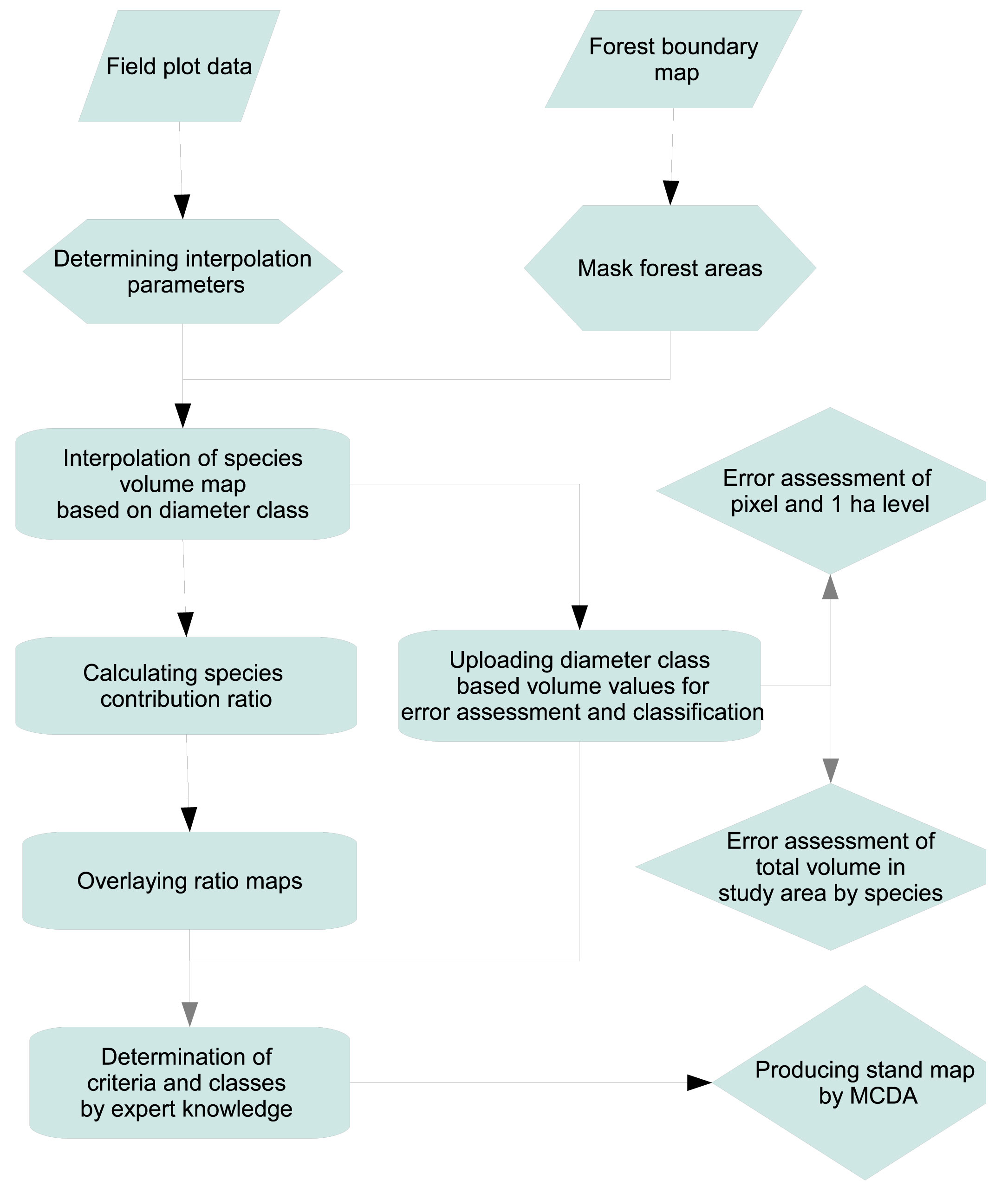
The vector and attribute data for the sample plots were entered into the GRASS GIS software database ([18], [59], [49]) in accordance with the methodological steps to produce an objective forest map (Fig. 2). The calculated volumes of tree species per ha were combined with the vector data. Eight different tree species occur in the study area. Of these eight species, the most common are Anatolian black pine, oak species, Oriental beech, and Calabrian pine (Tab. 1). Oak was present in 670 of 1050 plots in the b diameter class, and black pine was present in 564 of 1050 plots in the c diameter class. Black pine had the highest mean volume per ha (124.26 m3 ha-1) in the e diameter class, and the maximum volume per ha (549.65 m3 ha-1 - Tab. 1). Based on the data for the presence of species by diameter class in the survey plots, the seven most common species according to diameter class (Qb, Pnc, Pnb, Qc, Pnd, Pne, Foc) were selected to determine the spatial interpolation tension and the smoothing parameters of the RST interpolation method. These seven species and diameter classes were chosen because potential error in the class with the largest volume and number of sample points could potentially influence the entire evaluation.
Fig. 2 - Synopsis of the methodological steps carried out in this investigation.
Tab. 1 - Summary statistics for inventory data and error results. (MAE): Mean absolute error; (MAD): Mean absolute error/Mean.
| Tree species |
Diameter class |
Number sample plots |
Min | Max | Mean | Standard error |
MAE 400 m2 |
MAD 400 m2 |
MAE 1 ha |
MAD 1 ha |
|---|---|---|---|---|---|---|---|---|---|---|
| Black pine |
b | 555 | 0.28 | 142.43 | 14.5 | 21.09 | 0.37 | 0.03 | 1.65 | 0.11 |
| c | 564 | 3.16 | 348.4 | 64.14 | 61.03 | 1.61 | 0.03 | 7.55 | 0.12 | |
| d | 463 | 13.03 | 500.85 | 91.88 | 80.55 | 2.56 | 0.03 | 10.31 | 0.11 | |
| e | 299 | 30.56 | 549.65 | 124.26 | 84.84 | 2.54 | 0.02 | 11.07 | 0.09 | |
| Calabrian pine | b | 145 | 0.37 | 77.08 | 10.13 | 14.99 | 0.07 | 0.01 | 0.35 | 0.03 |
| c | 167 | 2.31 | 208.8 | 43.11 | 39.01 | 0.29 | 0.01 | 1.5 | 0.03 | |
| d | 131 | 1.3 | 373.28 | 79.04 | 67.08 | 0.51 | 0.01 | 2.47 | 0.03 | |
| e | 75 | 25.31 | 413.68 | 101.83 | 79.41 | 0.35 | 0 | 1.84 | 0.02 | |
| Other deciduous |
b | 166 | 0.44 | 23.63 | 4.94 | 4.74 | 0.06 | 0.01 | 0.3 | 0.06 |
| c | 49 | 3.06 | 51.1 | 11.29 | 9.96 | 0.05 | 0 | 0.24 | 0.02 | |
| d | 3 | 22 | 29.42 | 25.71 | 5.25 | 0 | 0 | 0.02 | 0 | |
| e | 2 | 34 | 34 | 34 | 0 | 0 | 0 | 0.02 | 0 | |
| Kazdagi fir |
b | 60 | 0.4 | 31.1 | 8.06 | 7.27 | 0.03 | 0 | 0.16 | 0.02 |
| c | 54 | 4.47 | 114.9 | 28.36 | 25.9 | 0.11 | 0 | 0.51 | 0.02 | |
| d | 29 | 22.73 | 191.53 | 63.73 | 41.75 | 0.14 | 0 | 0.67 | 0.01 | |
| e | 10 | 30.34 | 105.33 | 56.95 | 24.62 | 0.05 | 0 | 0.25 | 0 | |
| Horn Beam |
b | 12 | 0.58 | 27.63 | 9.38 | 9.8 | 0.01 | 0 | 0.05 | 0.01 |
| c | 6 | 4.5 | 34.83 | 17.41 | 11.5 | 0.01 | 0 | 0.04 | 0 | |
| d | 3 | 18 | 27 | 22.5 | 6.36 | 0 | 0 | 0.02 | 0 | |
| Oriental beech | b | 202 | 0.47 | 44.93 | 11.69 | 9.83 | 0.13 | 0.01 | 0.53 | 0.05 |
| c | 179 | 3.88 | 202.78 | 54.29 | 41.53 | 0.68 | 0.01 | 2.2 | 0.04 | |
| d | 98 | 14.4 | 360.27 | 60.56 | 51.64 | 0.48 | 0.01 | 1.74 | 0.03 | |
| e | 36 | 29.7 | 338.8 | 92.37 | 70.37 | 0.37 | 0 | 1.33 | 0.01 | |
| Spanish chestnut | b | 31 | 0.6 | 19.3 | 5.53 | 4.17 | 0.02 | 0 | 0.08 | 0.01 |
| c | 25 | 6.3 | 103.6 | 23.48 | 22.27 | 0.06 | 0 | 0.27 | 0.01 | |
| d | 7 | 17.63 | 60.1 | 37.33 | 14.3 | 0.02 | 0 | 0.11 | 0 | |
| e | 5 | 17.77 | 136.6 | 74.61 | 51.2 | 0.02 | 0 | 0.13 | 0 | |
| Oaks sp. | b | 670 | 0.44 | 70.85 | 11.89 | 11.35 | 0.35 | 0.03 | 1.61 | 0.14 |
| c | 514 | 2.71 | 148.75 | 30.55 | 25.19 | 0.72 | 0.02 | 3.2 | 0.10 | |
| d | 289 | 8.73 | 173.85 | 43.62 | 31.53 | 0.75 | 0.02 | 3.39 | 0.08 | |
| e | 158 | 17.85 | 240.25 | 65.46 | 45.29 | 0.71 | 0.01 | 3.43 | 0.05 |
Determining spatial interpolation parameters
To minimize the effects of prediction error and to determine the prediction parameters, different tension and smoothing parameters were tested using the “v.surf.rst” module (spatial approximation and topographic analysis from a given point or isoline data in vector format to floating point raster format using regularized spline with tension) of the GRASS software ([18]). The cross-validation and deviation values were calculated for the seven most common species by diameter class.
Cross-validation ([11]) was performed by dividing the data into two groups. The first group was used for interpolation using the method under evaluation. The second group was then used for comparison ([53], [54]). “Leave-one-out” cross-validation is a very common procedure and is frequently implemented in GIS packages. By minimizing the root-mean-square error (RMSE), cross-validation ensures that optimal interpolation parameters are found ([24]).
Prediction of forest map
Spatial interpolation methods transform data representing a continuous phenomenon in a vector point-and-line. This transformation involves mathematical functions allowed to pass through or near given points ([48]). Data collected for forest inventories are generally pinpoint-based because of the cost associated with the inventories. Pinpoint data are converted into continuous surfaces with the spatial interpolation functions implemented into the GIS package. Although many interpolation methods exist, GRASS software provides the analytic capability needed for methods such as Voronoi polygons, IDW and RSWT ([48]).
The changeable approach to intermediary estimation depends on the solution to the following problem: does the intermediary estimation function pass through or close to the data points, or can it be smoothed as much as possible? These two requirements are combined into a single condition to decrease the total deviation at the measured points and to smooth the spline function semi-norm ([44], [43]). Splines including the selection of the covariance function, as specified by numerous authors, are equivalent to universal kriging ([23], [48]).
Predictions based on the volume values per ha were obtained with the estimation parameters determined from the cross-validation and deviation method. This procedure (RST) is implemented within GRASS’s “v.surf.rst” module ([18]). Subsequently, the maps obtained were processed with particular GIS commands to produce the species contribution ratio maps and the mixture map.
Error assessment
The accuracy of the prediction maps computed with RST was calculated on both point and area basis. The MAE (Mean Absolute Error) and the MAD (Mean Absolute Deviation) were determined during the evaluation of the errors in the volume-estimation maps. The “v.sample” command was used to determine the point-wise error, and the “v.rast.stats” command was used to determine the area-wise error. The volumes (in ha) derived from the measured values from the inventory sampling plots in the field were compared with the predicted values at the applicable point on the maps obtained by interpolation. The area-based evaluation considered that each sample point represented precisely 1 ha. In addition, the total area-based volume was calculated and compared with the value obtained from conventional inventory methods.
Production of stand map from interpolation maps
The computed raster maps of the volume per ha for each species (Pb, Pn, Ab, Fo, Q, Cb, Cs, Od) were converted to vector maps and then overlaid to produce a vector map displaying the mixture ratios of the 8 species. The combinations acquired from these maps were evaluated with expert knowledge of forest management. This evaluation was then used to determine the criteria and classes for making the final decision map for the managed forest. For example, in Tab. 2, 8 species and diameter class combinations were categorized into a single category by defined expert knowledge criteria. All other similar combinations were categorized with this approach. This procedure used the ELECTRE TRI “Bouyssou-Marchant” model in Quantum GIS ([52], [57]).
Tab. 2 - ELECTRE TRI categorization sample.
| 1. 6Pn2Fo1Q1Cb de | 6Pn2Fo1Q1Cb de |
| 2. 6Pn2Fo1Q1Cb de | |
| 3. 6Pn3Fo1Q de | |
| 4. 6Pn2Fo2Q de | |
| 5. 6Pn2Fo2Q ed | |
| 6. 6Pn2Fo1Q1Cb ed | |
| 7. 6Pn1Fo2Q1Cb d | |
| 8. 6Pn2Fo2Cb de |
Results
Determining spatial interpolation parameters
Based on the cross-validation results obtained in this study, the interpolation parameters showing the lowest RMSE value varied among the seven diameter classes considered (Tab. 3). Therefore, a map showing the deviation of the seven most common species by diameter class was calculated. All diameter classes gave the minimum mean absolute-deviation error, with a value of 80 for the tension parameter and a value of 0.2 for the smoothing parameter (Tab. 3). The use of these values for interpolation would likely decrease the error rate.
Tab. 3 - Deviation values for the seven most common species by diameter class.
| Tree Species |
Cross validation | Deviation | Smoothing | ||||||
|---|---|---|---|---|---|---|---|---|---|
| 20 | 40 | 60 | 80 | 20 | 40 | 60 | 80 | ||
| Pnb | 6.64 | 6.6 | 6.6 | 6.6 | 0.39 | 0.26 | 0.22 | 0.2 | 0.2 |
| 6.63 | 6.6 | 6.6 | 6.6 | 0.72 | 0.49 | 0.42 | 0.38 | 0.4 | |
| 6.62 | 6.6 | 6.6 | 6.6 | 1 | 0.71 | 0.61 | 0.55 | 0.6 | |
| 6.61 | 6.6 | 6.61 | 6.61 | 1.26 | 0.91 | 0.78 | 0.72 | 0.8 | |
| Pnc | 30.36 | 30.29 | 30.35 | 30.4 | 1.83 | 1.23 | 1.04 | 0.93 | 0.2 |
| 30.32 | 30.3 | 30.36 | 30.42 | 3.36 | 2.32 | 1.98 | 1.79 | 0.4 | |
| 30.29 | 30.31 | 30.38 | 30.44 | 4.69 | 3.32 | 2.85 | 2.59 | 0.6 | |
| 30.28 | 30.33 | 30.4 | 30.46 | 5.87 | 4.23 | 3.66 | 3.35 | 0.8 | |
| Pnd | 39.66 | 39.4 | 39.37 | 39.37 | 2.38 | 1.59 | 1.34 | 1.2 | 0.2 |
| 39.58 | 39.38 | 39.36 | 39.37 | 4.38 | 3 | 2.55 | 2.31 | 0.4 | |
| 39.52 | 39.37 | 39.36 | 39.38 | 6.12 | 4.3 | 3.68 | 3.35 | 0.6 | |
| 39.47 | 39.36 | 39.36 | 39.39 | 7.65 | 5.49 | 4.73 | 4.32 | 0.8 | |
| Pne | 43.38 | 42.92 | 42.84 | 42.82 | 2.73 | 1.8 | 1.51 | 1.35 | 0.2 |
| 43.23 | 42.88 | 42.83 | 42.81 | 4.98 | 3.38 | 2.86 | 2.58 | 0.4 | |
| 43.13 | 42.86 | 42.81 | 42.8 | 6.92 | 4.82 | 4.11 | 3.73 | 0.6 | |
| 43.05 | 42.84 | 42.8 | 42.79 | 8.63 | 6.14 | 5.27 | 4.8 | 0.8 | |
| Foc | 8.5 | 8.49 | 8.53 | 8.57 | 0.53 | 0.35 | 0.29 | 0.27 | 0.2 |
| 8.48 | 8.5 | 8.55 | 8.58 | 0.98 | 0.67 | 0.57 | 0.51 | 0.4 | |
| 8.47 | 8.51 | 8.56 | 8.59 | 1.37 | 0.96 | 0.82 | 0.75 | 0.6 | |
| 8.46 | 8.52 | 8.57 | 8.61 | 1.71 | 1.22 | 1.06 | 0.97 | 0.8 | |
| Qb | 6.5 | 6.42 | 6.41 | 6.4 | 0.4 | 0.26 | 0.22 | 0.2 | 0.2 |
| 6.47 | 6.41 | 6.4 | 6.4 | 0.73 | 0.5 | 0.42 | 0.38 | 0.4 | |
| 6.46 | 6.41 | 6.4 | 6.4 | 1.01 | 0.71 | 0.61 | 0.55 | 0.6 | |
| 6.44 | 6.41 | 6.4 | 6.41 | 1.26 | 0.9 | 0.78 | 0.71 | 0.8 | |
| Qc | - | - | - | - | 0.78 | 0.52 | 0.43 | 0.39 | 0.2 |
| - | - | - | - | 1.44 | 0.98 | 0.83 | 0.75 | 0.4 | |
| - | - | - | - | 2 | 1.4 | 1.2 | 1.09 | 0.6 | |
| - | - | - | - | 2.5 | 1.78 | 1.54 | 1.4 | 0.8 | |
Prediction of forest maps
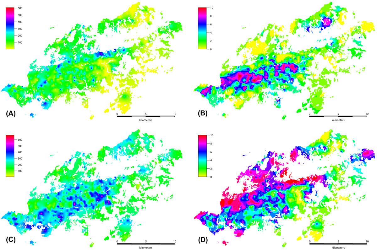
A total of 31 independent interpolation maps were obtained for the diameter classes of each species (e.g., black pine in Fig. 3a, b, c, and d). The total volumes of particular species per ha (e.g., black pine: Pnb + Pnc + Pnd + Pne = Pnt) were computed by summing these species-diameter-class interpolation maps (Fig. 4a). The percentage contributions of each diameter class to the mixture were obtained by calculating the ratios of the diameter class volume of the particular species and the total volume of the species (e.g., Pnb/Pnt) with the help of this map (Fig. 4b). Similarly, the summation of the total volumes of each species per ha (Pnt + Pbt + Odt + Abt + Cbt + Fot + Cst + Qt = Vt) yielded the total volume per ha of the trees in the planning units (Fig. 4c). The percentage contributions of each species to the mixture were obtained by calculating the ratios of the total volume of the species and the overall total volume (e.g., Pnt/Vt) with the help of this map (Fig. 4d).
Fig. 3 - Interpolation maps of black pine. (A) diameter class; (B) diameter class ; (C) diameter class ; (D) diameter class
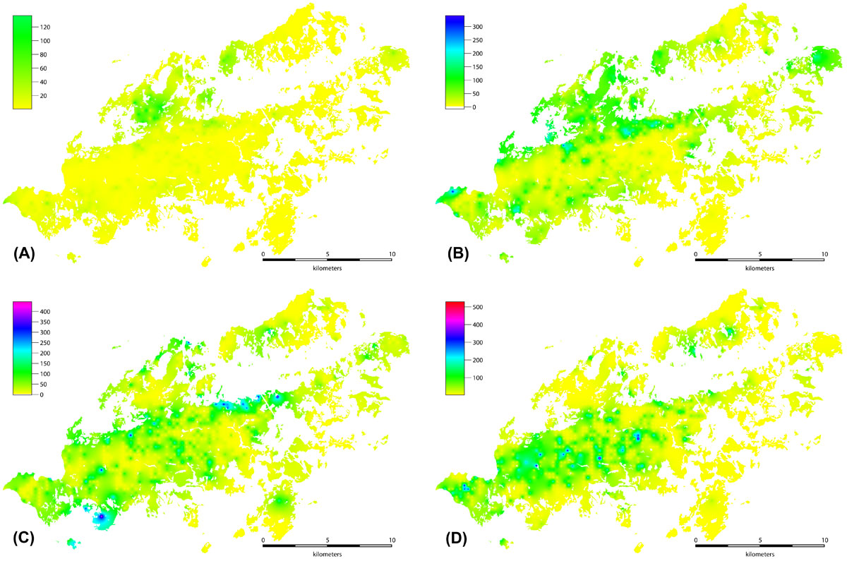
Fig. 4 - (A) Total volume map for black pine; (B) volume ratio map for black pine (diameter class b); (C) total volume map for all the species; (D) volume ratio map for black pine.
Error assessment of predictions
If the predictions were evaluated on the basis of the size of one pixel (400 m2), the results were very satisfactory (MAD < 4%). However, on the basis of a sample plot that was approximately one ha in area, the maximum MAD increased to 12% (Pnb) and 14% (Qb). The maximum standard deviations for the black-pine diameter classes d and e, were 81% and 85%, respectively (Tab. 1). High standard deviations were also found for the Calabrian-pine diameter classes d and e (67% and 79%, respectively), Oriental beech (51% and 70%, respectively), and oak spp. (31% and 45%, respectively).
The total volume by species as determined by conventional methods ([15]) and was compared to that determined by the methods applied in our study for the entire study area (Tab. 4). The data over the entire area showed that four species had volume ratios greater than 1%. In descending order of volume ratios, these species were Pn > Q > Pb > Fo, with volume ratio values of 55%, 19%, 16%, and 8%, respectively. These four species represented a total volume of 98%. The maximum relative errors were calculated for the Calabrian pine diameter classes b and c. These relative error values were +33% and +23%, respectively. The minimum relative errors for these four species were calculated for diameter classes b, c, and d of the oak species. These relative error values were 2%, 4%, and 2%, respectively.
Tab. 4 - Accuracy of total volume calculated with spatial interpolation (SI), compared with conventional forest inventory results (CFIR).
| Tree species |
Type of estimation |
Diameter | Total contribution |
Total partecipant | |||
|---|---|---|---|---|---|---|---|
| Class b | Class c | Class d | Class e | ||||
| Pb | SI | 36226 | 165430 | 248434 | 220339 | 670428 | 0.16 |
| CFIR | 27332 | 134388 | 211765 | 180807 | 554292 | ||
| % | 33 | 23 | 17 | 22 | 21 | ||
| Pn | SI | 146309 | 611316 | 695638 | 559590 | 2012853 | 0.55 |
| CFIR | 160647 | 529222 | 614516 | 625805 | 1930190 | ||
| % | -9 | 16 | 13 | -11 | 4 | ||
| Ab | SI | 5507 | 15973 | 20363 | 5326 | 47169 | 0.01 |
| CFIR | 4273 | 12838 | 16481 | 6034 | 39626 | ||
| % | 29 | 24 | 24 | -12 | 19 | ||
| Fo | SI | 34856 | 141304 | 95689 | 52129 | 323978 | 0.08 |
| CFIR | 31873 | 128509 | 80135 | 44008 | 284525 | ||
| % | 9 | 10 | 19 | 18 | 14 | ||
| Q | SI | 132299 | 233543 | 176357 | 150154 | 692353 | 0.19 |
| CFIR | 132519 | 228881 | 170362 | 147514 | 679276 | ||
| % | 0 | 2 | 4 | 2 | 2 | ||
| Cb | SI | 1111 | 1023 | 710 | 0 | 2845 | 0 |
| CFIR | 1101 | 871 | 576 | 0 | 2548 | ||
| % | 1 | 17 | 23 | - | 12 | ||
| Cs | SI | 2367 | 7859 | 3324 | 4979 | 18529 | 0 |
| CFIR | 2092 | 7351 | 2759 | 2035 | 14237 | ||
| % | 13 | 7 | 20 | 145 | 30 | ||
| Od | SI | 13044 | 9291 | 1333 | 785 | 24452 | 0.01 |
| CFIR | 12228 | 7363 | 2414 | 257 | 22262 | ||
| % | 7 | 26 | -45 | 205 | 10 | ||
Black pine had a maximum volume ratio of 55% for the entire study area and a total relative error of 4%. The relative error rates for the individual diameter classes were 16% for class c, 13% for class d and -11% for class e.
Oriental beech has the lowest volume ratio (8%) of the four highest-volume species. The relative error for the total volume was 14%. The relative errors for the diameter classes were 10%, 19%, and 18% for classes c, d, and e, respectively.
Generally, the highest relative errors in volume estimation occurred for diameter classes c and d.
The pixel-based (sampling area-based) MAE and the area-based MAE followed similar trends. The pixel-based MAD values ranged between 0% and 3%.
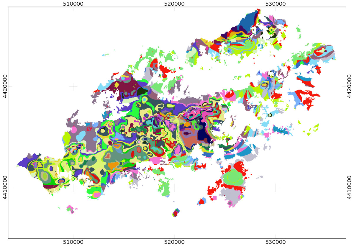
When producing the forest stand map from the interpolation maps, the diameter class for each value of species volume derived from the raster maps was uploaded with the “v.rast.stats” command onto the vector map as attribute data. The resulting species mixtures, including both volume-based dominants and accompanying secondary species, were then considered. In the next stage of the process, the 890 different mixture variations were reduced to a smaller number of categories based on expert knowledge. Criteria were established based on the mixture rates of the tree species and the average volumes for the diameter classes. These ELECTRE TRI criteria and the values for the weights were then entered, and 70 different profiles were generated. The ELECTRE TRI module of QGIS was used to create a final decision map. This map represents 70 different profile categories based on species mixture rates and diameter classes (Fig. 5).
Fig. 5 - Stand type maps obtained using the ELECTRE TRI approach by combining the 31 prediction maps of the volume per ha.
Discussion
Diameter classes d and e showed the larger standard devistions for species representing 98% of the total volume (Tab. 1). In general, the observed error values were as low as expected from the associated standard deviations, with occasional exceptions. Minor differences were found between MAD errors at the pixel level and at the 1-ha level.
The observed differences in MAE among diameter classes for the same species could be interpreted as due to variation in site index between neighboring plots, that could cause the volume to increase by approximately 15%. Moreover, differences in canopy closure between neighboring stands could have also contributed to the observed differences in MAE described above. Therefore, MAE could be reduced by including the above parameters in the volume estimation, although the number of maps to be produced would also increase.
In the species diameter class with approximately 300 observations distributed around a value of about 300, the MAD values calculated on the basis of 1 ha were 8% and 9% for Qd and Pne, respectively. Increasing the number of species found at the sampling points (Qb, Pnc, Pnb, Pnd, and Qc), the same trend was observed. This increase in the error values is not affected by standard deviation or mean volume (Tab. 1). These maximum MAD values could result from the distribution of black pine and oak species in the study area. Indeed, data heterogeneity may fairly affect the performance of the methods ([38]).
The design of the RST method adopted in this study ensures that the predicted values at a given points remain very close to the observed values at that point. Thus, the MAD of the sampling plots (400 m2 = 1 pixel) did not increase at the ha level (10 000 m2/400 m2=25 pixels). This result reflects the characteristics of the inventoried sample plots, whose structure was fairly similar to the forest structure in the surrounding area.
The volumes obtained by the RST method were slightly higher than the corresponding values in the forest management plan data (Tab. 4). Black pine showed the highest volume ratio (55%), with a relative error of 4% only. The largest error value was detected for diameter class b of Calabrian pine. The observed differences can be accounted for by differences between the two methods. The classical method adopted in forest management plans evaluates the data groups separately to create separate stand types. Instead, the spatial interpolation approach used here evaluates the data relative to the overall configuration of the observations and the spatial scales. Different results are also expected because of the subjective personal evaluations involved in conventional approaches.
According to the 2008 Turkish Forest Management Regulation Handbook ([15]), an error ≤ 10% in volume assessment would be expected for production forests. However, unlike production forests, an error rate > 10% is accepted for protected forests because each systematic sampling point is 600 x 600 m = 36 000 m2. Thus, based on the above criteria, the results of this study could be considered as acceptable.
In this study, a final decision map has been produced representing 70 different profile categories based on species mixture rates and diameter classes in the area analyzed (Fig. 5), obtained combining the prediction maps produced. The method adopted has facilitated the reductions performed for adjacent diameter classes. In addition, the small forest fragments were integrated into a general framework by the analysis. Therefore, this approach facilitated the reduction of small fragments until the structural and statistical features of the desired stand types were attained, in accordance with management goals. To perform this reduction process in a objective way, the ELECTRE TRI method was used. Aktas & Yilmaz ([2]) also used the same methodology to produce a stand map from interpolation maps. The above process would require the use of expert knowledge on forest management to make an improved decision map.
The area considered in this study enlarged upon both forested and non-forested zones (e.g., agricultural areas, settlements, and grasslands). To avoid the effect of the latter areas on total volume assessment, adequate masks were used to exclude non-forested area from the analysis. An additional problem encountered is the accuracy of predictions near the boundaries of the forest management units. The incorporation of neighboring plan units in these areas is an appropriate way of improving the accuracy of predictions. Nevertheless, the resulting map should be refined through aerial photography or satellite images.
Spatial interpolation methods (especially kringing) have been previously argued as unsuitable for assessment purposes in managed forests ([1]). On the other hand, several studies have reported successful application of such methods in homogenous natural forest areas ([20], [62]).
The RST method adopted here allows the user to create stand maps very efficiently. In order to test the accuracy of volume predictions, cross-validation and resampling methods have been applied ([47], [66], [50], [58], [33], [60], [63]), aimed at comparing the observed value at a given point with its prediction obtained from the interpolated continuous surface. However, in areas characterized by highly heterogeneous forest structures, the above approach may not be adequate, and additional control points in the field may be required. On the contrary, a subset of sampling points may be used in areas densely sampled for the above comparisons, keeping the points excluded from analysis for control purposes.
Further improvement of the map obtained may be achieved by the inclusion of auxiliary data (e.g., soil, climate, topography etc.) and the use of multivariate interpolation methods or mixed models, thus combining the most important parameters of the forest stands. For example, several environmental parameters have been used to model the spatial variability in Pinus radiata productivity in New Zealand ([32]). Moreover, remote sensing data may be incorporated into the analysis to obtain an improved accuracy of predictions. Dubayah et al. ([9]) found that the LiDAR remote sensing has a vast potential for the direct estimation of several key forest characteristics, such as canopy heights, stand volume, basal area and aboveground biomass ([8]). Lovell et al. ([39]) have performed studies on optimal LiDAR acquisition parameters for forest height retrieval. Estornell et al. ([12]) have made estimations of shrub biomass by airborne LiDAR in small forest stands, obtaining accurate measures of the most important plant parameters (volume, average height, diameter and canopy) with minimal costs. Haywood ([21]) adopted a semi-automated stand delineation process in the mapping of natural eucalypt forests using remote sensing, multi-spectral imagery, lasers and stand characteristics. Furthermore, the application of LiDAR allows the creation of accurate three-dimensional relief models of forest stands. For example, Mitasova et al. ([45]) used a simultaneous spline approximation and topographic analysis for LiDAR elevation data in open-source GIS to create accurate relief models. LiDAR, in combination with inventory data, has also been used to evaluate the forest habitats of birds and other wildlife ([17], [61], [65], [56]).
Forest management activities depends on international, national, and regional forestry strategies. Moreover, regional planning should include community participation and the analysis of multiple functions of forest resources ([51]). For this reason, multi-function criteria are often used in forest planning in addition to conventional management criteria, and MCDA has been carried out in different decision-making contexts in forestry. Khadka & Vacik ([31]) used multi-criteria analysis to support community forest management including 6 criteria and 40 profiles. Huth et al. ([26]) used multi-criteria analysis to support decisions on harvest volume based on the criteria of rotation, harvest intensity, and target diameter.
In many forestry studies, MCDA was applied using multiple criteria for the assessment of a single parameter (e.g., total volume, site class). Similarily, the MCDA map obtained in our study has also multiple criteria and allows the evaluation of multiple functions. The conventional methods used in Turkey require professional experience and a background of appropriate knowledge. The use of an MCDA method, such as the ELECTRE TRI adopted here, may bypass the above problem.
References
Gscholar
Gscholar
Gscholar
Gscholar
Gscholar
Gscholar
Gscholar
Gscholar
Gscholar
Gscholar
Gscholar
Gscholar
Gscholar
Gscholar
Gscholar
Gscholar
Gscholar
Gscholar
Gscholar
Gscholar
Authors’ Info
Authors’ Affiliation
Department of Forest Management, Faculty of Forestry, Istanbul University, 34473 Bahçeköy, Istanbul (Turkey)
Department of Forest Engineering, Faculty of Forestry, Istanbul University, 34473 Bahçeköy, Istanbul (Turkey)
Department of Forest Management, Regional Forest Directorate of Istanbul, Istanbul (Turkey)
Corresponding author
Paper Info
Citation
Destan S, Yilmaz O, Sahin A (2013). Making objective forest stand maps of mixed managed forest with spatial interpolation and multi-criteria decision analysis. iForest 6: 268-277. - doi: 10.3832/ifor0099-006
Academic Editor
Agostino Ferrara
Paper history
Received: May 18, 2012
Accepted: Mar 18, 2013
First online: Jul 01, 2013
Publication Date: Oct 01, 2013
Publication Time: 3.50 months
Copyright Information
© SISEF - The Italian Society of Silviculture and Forest Ecology 2013
Open Access
This article is distributed under the terms of the Creative Commons Attribution-Non Commercial 4.0 International (https://creativecommons.org/licenses/by-nc/4.0/), which permits unrestricted use, distribution, and reproduction in any medium, provided you give appropriate credit to the original author(s) and the source, provide a link to the Creative Commons license, and indicate if changes were made.

Web Metrics
Breakdown by View Type
Article Usage
Total Article Views: 60704
(from publication date up to now)
Breakdown by View Type
HTML Page Views: 49260
Abstract Page Views: 4235
PDF Downloads: 5543
Citation/Reference Downloads: 25
XML Downloads: 1641
Web Metrics
Days since publication: 4764
Overall contacts: 60704
Avg. contacts per week: 89.20
Article Citations
Article citations are based on data periodically collected from the Clarivate Web of Science web site
(last update: Mar 2025)
Total number of cites (since 2013): 9
Average cites per year: 0.69
Publication Metrics
by Dimensions ©
Articles citing this article
List of the papers citing this article based on CrossRef Cited-by.
Related Contents
iForest Similar Articles
Research Articles
Use of multi-criteria analysis (MCA) for supporting community forest management
vol. 5, pp. 60-71 (online: 12 April 2012)
Research Articles
Distribution of the major forest tree species in Turkey within spatially interpolated plant heat and hardiness zone maps
vol. 5, pp. 83-92 (online: 30 April 2012)
Review Papers
The role of spatial criteria in enhancing forest restoration actions: a systematic review
vol. 19, pp. 157-167 (online: 11 May 2026)
Review Papers
Integration of forest mapping and inventory to support forest management
vol. 3, pp. 59-64 (online: 17 May 2010)
Commentaries & Perspectives
Benefits of a strategic national forest inventory to science and society: the USDA Forest Service Forest Inventory and Analysis program
vol. 1, pp. 81-85 (online: 28 February 2008)
Research Articles
Using self-organizing maps in the visualization and analysis of forest inventory
vol. 5, pp. 216-223 (online: 02 October 2012)
Research Articles
Application of indicators network analysis to support local forest management plan development: a case study in Molise, Italy
vol. 5, pp. 31-37 (online: 27 February 2012)
Research Articles
Usefulness and perceived usefulness of Decision Support Systems (DSSs) in participatory forest planning: the final users’ point of view
vol. 9, pp. 422-429 (online: 02 January 2016)
Research Articles
Biomasfor: an open-source holistic model for the assessment of sustainable forest bioenergy
vol. 6, pp. 285-293 (online: 01 July 2013)
Research Articles
The analytic hierarchy process for selection of suitable trees for Mexico City
vol. 13, pp. 541-547 (online: 18 November 2020)
iForest Database Search
Search By Author
Search By Keyword
Google Scholar Search
Citing Articles
Search By Author
Search By Keywords
PubMed Search
Search By Author
Search By Keyword


