A Decision Support System for trade-off analysis and dynamic evaluation of forest ecosystem services
iForest - Biogeosciences and Forestry, Volume 11, Issue 1, Pages 171-180 (2018)
doi: https://doi.org/10.3832/ifor2416-010
Published: Feb 19, 2018 - Copyright © 2018 SISEF
Research Articles
Abstract
This paper presents an open-source Decision Support System (DSS) able to quantify the economic value of forest ecosystem services and their dynamic trade-offs. Provisioning, regulation and support services, as well as cultural services, can be evaluated by the model. Best management forestry practices can be identified by optimizing specific objective functions, e.g., maximizing the economic value or identifying the ideal rotation period. The model was applied to a silver fir (Abies alba Mill.) stand in central Italy as a case study. Results show the importance of economic parameters (e.g., discount rate) and management practices (e.g., presence/absence of silvicultural thinning) in defining forest values. The main strengths and weaknesses of the DSS are discussed in light of its potential for application in the sector of Payment for Ecosystem Services.
Keywords
Ecosystem Services Planning, Complex Systems Analysis, Systemic Rotation Period, Nonlinear Programming
Introduction
Starting from the pioneering work of Costanza et al. ([10]), several attempts have been made to calculate the monetary value of ecosystem services (ES) and its change over time ([21], [11]). The quantification and integrated evaluation of these functions are in fact considered a cornerstone for natural resources planning and scenario analysis ([23]). Among the different techniques for ES evaluation, monetization is the most applied because it can be used for Cost-Benefit Analysis (CBA). In CBA, market and non-market benefits and costs are appraised in economic terms, allowing for comparison of management alternatives by means of either the Net Present Value (NPV) or the capital value ([1]).
The concept of ES evolved with the development of monetary valuation techniques ([38]). In particular, the term was coined as a metaphor to appeal to public opinion ([36]) and to best define general concepts such as the “multifunctionality” of environmental goods and services. In TEEB ([47]), ES are defined as the direct and indirect contributions of ecosystems to human wellbeing or, in economic terms, the “dividend” that society receives from natural capital. Different methodologies have been applied to determine the relative importance of single ecosystem services or the Total Economic Value (also defined as Total Value of Ecosystem Services - TVES). Estimates vary widely, depending on context ([35]).
To review the scientific literature on the monetization of ES, De Groot et al. ([14]) compiled an Ecosystem Service Value Database (ESVD) containing more than 1350 estimates. Most studies have calculated the economic value of ES using preference methods, such as the Contingent Valuation technique or Choice Experiments ([20], [27]), or revealed preferences approaches, i.e., the Travel Cost method ([3], [30]) or Hedonic Pricing method ([56], [12]). Benefit Transfer has also been applied extensively ([53], [46], [41]). The limitations of these methods have been illustrated and amply discussed in the literature ([32], [7], [2]), including suggestions for their improvement. Analyzing the limitations of the above-mentioned methodologies is beyond the scope of this work; for details, see Gsottbauer et al. ([19]).
Despite the importance of ES economic quantification, research and empirical examples highlight the main difficulties in monetizing ES. The definition of ES and their classification (such that environmental functions are not accounted for more than once) is a major issue ([25], [34]). Another difficulty lies in quantifying the TVES. The TVES is often calculated as the simple sum of ES values ([13]), without taking into consideration neither the analysis of trade-offs nor the competitive and complementary nature of ES ([35]).
In the case of forest ES, calculating the TVES is of great importance in forest governance ([45]). Unfortunately, it is often calculated in static terms, ignoring the dynamic nature of stands and the possible impact of disservices and disturbances on ES (e.g., damage to wildlife and storms). A number of studies have focused on the dynamic analysis of forest ES and on determining their economic value. Häyhä et al. ([22]) used a Geographic Information System (GIS) to evaluate trade-offs among different ES, whereas Rose & Chapman ([42]) provided additional insights into ES estimation. The latter have implemented a method to define the optimal stand age for maximizing the Net Present Value (NPV) of multiple ES. Trade-off evaluation among forest ES is influenced by the spatial-temporal scale of analysis ([54]). A DSS should facilitate multiscale approaches (in particular from the spatial point of view) so that the effects of forest management (e.g., from good production to landscape improvement) can be taken into account. The literature mainly focuses on large/medium-scale assessment of ES trade-offs. For example, Mazzaro De Freitas et al. ([33]) evaluated the different offsetting implementation practices and their effects on nature conservation and socio-economic development in Brazil. Bottalico et al. ([6]) used an integrated GIS-based approach for scenario analysis and economic valuation of wood production and carbon sequestration trade-offs in forests of the Molise region (Italy).
Two main economic biases are present in the literature on ES monetization. First, several works are based on the assumption of Turner et al. ([50]) that the marginal value of ES is relevant for economic quantification. Indeed, marginal values can provide a good approximation of ES variations. However, in the case of market exchanges and trade between buyers and sellers, the total value of ES must be taken into account. For example, when a forest compartment is sold, the total value should be considered and not just the variations in the flux of ES or in marginal utility. The second bias stems from the use of NPV in economic analysis, a method widely applied in environmental economics, as the NPV is calculated for a limited period of investment. However, the effects of forest assessment and management are not limited to just one rotation period. This is demonstrated by the fact that forest economics and appraisal historically take into account the Faustmann’s Rule for forest estimation ([15]). Faustmann’s formula quantify the present value of bare land for a specific forest. This value derives from the capitalization of periodic forest income obtainable in a rotation period. Faustmann noted that the marginal costs of delaying harvests include both foregone interest payments and the loss of value due to delayed rotation ([8]). This means that the economic value of forest ES should be quantified as capitalized value and not as NPV.
Furthermore, there is a gap between existing Decision Support Systems (DSS) for management/monetary evaluation of forests and the requirements of end-users ([55]). Bagstad et al. ([4]) completed a detailed literature review of existing DSS for assessing, quantifying, modeling, valuing and/or mapping ES. The study describes 17 ES tools and assesses their “readiness” for application in the decision-making processes. One specific assessment looks at the ability to monetize ES.
To overcome the above-mentioned limitations, an open-source DSS was developed which could be applied in: (i) the analysis of forest ES trade-offs; and (ii) the optimization of forest management in order to maximize the economic value of ES. The proposed model quantifies the trade-offs among ES for different economic and management variables. So far, the few studies on this topic in the literature have usually analyzed no more than two ES each. An additional strength of the proposed model is its optimization of ES values through a nonlinear programming procedure. Specific objective functions such as maximization of the monetary or biophysical value of ES can be defined by modifying specific input data and parameters.
Methodology
The DSS evaluation criteria are those suggested by Bagstad et al. ([4]). The model was developed in spreadsheet form and consists of three sections: input, processing and output.
Model approach and data input
Basic information on forest stand characteristics and ES categories is provided in the input page. The rotation period is set to a preliminary value. There are two possible management options (high forest and coppice) with different potential yields in the final cut (0-100%, e.g., to consider release of standards in coppices). Thinning intervention and the age of thinning are additional options. Site parameters are slope, distance from roads and soil fertility.
Dynamic assessment of forest characteristics is used to determine trade-offs among ES. In this respect, additional input can be provided by yield tables for even-aged stands, or norms for uneven-aged forests. Yield tables are applied to establish polynomial functions suitable for calculating the total volume and mean diameter. These variables are differentiated according to the presence or absence of thinning.
TOOFES applies the commonly used TEEB ([47]) classification of ES, which considers four different groups: (i) provisioning; (ii) regulating; (iii) habitat or supporting; and (iv) cultural services. Each category comprises a series of specific subcategories ([47]) such as (i) provisioning services: food, fresh water, raw materials, medicinal resources; (ii) regulating services: local climate and air quality regulation, carbon sequestration and storage, moderation of extreme events, waste-water treatment, erosion prevention and maintenance of soil fertility, pollination, biological control; (iii) habitat or supporting services: habitats for species, maintenance of genetic diversity; (iv) cultural services: recreation and mental and physical health, tourism, aesthetic appreciation and inspiration, spiritual experience and sense of place. Although only one category per class was considered in testing the model, the structure of the DSS can easily be updated with additional ES functions.
Provisioning services are here connected to raw materials production. In short, the discount rate and one to three wood categories (differentiated by diameter) can be input. A selling price can be defined (assuming sale at the landing site) for each category. Production costs take into account productivity and the unitary costs of labor and machinery for felling trees and extracting wood, as well as general expenses (direction costs, administrative costs and interest on advanced capital).
Regulating services focus on carbon sequestration. Calculations are based on the annual increment, taking into account carbon accumulated in biomass above and below ground. The annual contribution of other carbon pools such as litter, deadwood and organic soil is considered negligible, because variations in carbon content are detected in the very long term ([22]). The variables used for quantification of stored carbon are the volume of growing stock, the Biomass Expansion Factor (BEF), Wood Basic Density (WBD) and the root/shoot ratio (R - [17]). The financial parameter is the price of carbon.
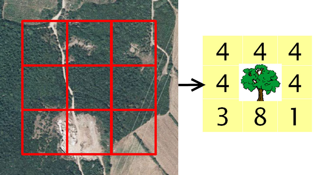
The value of supporting services focuses on the analysis of biodiversity in the examined forests. Pearce & Moran ([37]) define biodiversity as genetic, species and ecosystem diversity. The literature contains several examples of forest biodiversity analyses for each of these categories (see [5] for a literature review). It is harder to complete a dynamic analysis of this component in one or more forest life cycles ([52]). Moreover, flexible DSS able to quantify the economic variability of biodiversity are not present in the literature. To overcome these difficulties, a method based on ecosystem diversity was adopted in TOOFES. Ecosystem diversity is an easier parameter to compute in respect of genetic and species diversity. Ecosystem diversity can be calculated in relation to land use modification and, as a consequence, to pattern analysis ([24]). It is usually evaluated using Geographic Information System (GIS) because such platforms can be used to automatically quantify several diversity indexes. In order to execute all operations in a single model, TOOFES applies a spreadsheet, cell-based procedure for pattern analysis. An example of input data for ecosystem diversity analysis is represented in Fig. 1. A 3 × 3 kernel shows land use for the eight cells around the analyzed forest. Land categories are: (1) agricultural area; (2) young coppice (<5 years old); (3) intermediate coppices (5-20 years old); (4): mature coppices (>20 years old); (5) young high forests (<10 years old); (6) intermediate high forest (10-50 years old); (7) mature high forests (>50 years old); (8) artificial surfaces, bare rocks, glaciers and perpetual snow, wetlands, water bodies. Each of the above classes have a different visual impact and habitat suitability. Classification can be completed through either photointerpretation or field evaluation. Patterns in raster images are necessarily simplified with respect to real ones (Fig. 1).
Fig. 1 - Example of pattern analysis for the studied forest (central cell).
An additional factor that must be taken into account is the economic value of biodiversity (biodτ) as derived from a Benefit Transfer approach or from ad hoc studies.
Cultural service is based on monetary quantification of touristic and recreational value. This value is often calculated in static terms. For example, the value of a forest at year x (commonly calculated through Choice Experiment, Contingent Valuation or Travel Cost methods) is not necessary the same for different forest ages.
The perceived touristic and recreational value of an environment does not seem to be a permanent construct but must be seen in the context of experiences and goods/service variations over time. It depends on personal experience and emotions ([26]). Quantification of these values should therefore take into account the entire life cycle of a forest or comparison among forests of different ages. To address this issue a method that correlates a dendrometric parameter with the cultural value is proposed. Ribe ([39]) confirmed the hypothesis that if other forest stand and facility characteristics do not vary, there is a direct proportion between dendrometric variables (in particular mean tree diameter) and touristic-recreational value. The inputs for calculating cultural significance are therefore: (i) the monetary value of touristic-recreational utility, as determined using a Benefit Transfer approach or from ad hoc research; and (ii) the age of the forest at the time of data collection.
Processing
The “Processing” section represents the core of the DSS. Dendrometric variables can be calculated using polynomial functions derived from yield tables. The volume of a forest (m3 ha-1) at a given year is determined as follows (eqn. 1):
where a, b and c are the estimated coefficients and x is the age of the forest.
Based on a similar approach, the mean diameter of a stand is calculated as (eqn. 2):
where Φx is the mean diameter (cm) at year x, and d, e and f are the estimated coefficients.
The market value of raw material is calculated as stumpage value for both final felling and thinning. It depends on the possible assortment types, their prices and production costs. Stumpage value is quantified following the methodology presented by Sacchelli et al. ([43]). The revenues ρ obtained from the stand at year x are calculated as (eqn. 3):
where i is the number of wood assortments, pi the average market price of the i-th assortment (€ m-3) and λ the percentage of extracted volume for silvicultural treatment v at year x.
For the α-th phase of the production process, the costs K at age x are calculated as (eqn. 4):
where kα is the hourly cost for the α-th process phase (€ h-1) and ηα is the hourly productivity for the α-th process phase (m3 h-1).
The hourly cost includes machinery and labor (3rd and 5th level) costs. For each phase the DSS defines the organization of the production process and calculates hourly productivity based on a prescribed yield, slope, and tree characteristics (volume and diameter), as well as the extraction distance. The direction cost Dx, administrative expense Adx and interest Ix are also calculated to determine the total cost ([43]).
Lastly, the value of provisioning services (VPS) is determined using the Faustmann’s formula ([15] - eqn. 5):
where ω is the rotation period of the forest (year),r is the discount rate, w the annual revenue (€ ha-1 year-1), S the renovation cost (€ ha-1), z the annual cost (€ ha-1 year-1) and s the forest area (ha).
The value of regulating services (VRS) due to carbon sequestration is defined as the capitalized value of carbon stored yearly in above- and below-ground biomass. The amount of carbon sequestered in trees is calculated through the procedure proposed by Federici et al. ([17]). The authors quantify total carbon tons at year x in above-ground (CAG,x) and below-ground (CBG,x) dry biomass using the following equations (eqn. 6, eqn. 7):
where vx-vx-1 represents the annual volume increment at year x (m3 ha-1 year-1). VRS is therefore (eqn. 8):
where ψ is the biomass/carbon conversion factor (t/t of dry matter) and σ the carbon price (€ t-1) reported in the database of the Euro-Mediterranean Centre on Climate Change ([9]).
Biodiversity is determined by pattern analysis based on relative richness ([49]). Taking into account the square matrix presented above, diversity in the examined forest at year x (χx) is calculated as follows (eqn. 9):
where nx is the number of different classes present in the kernel at year x, and MAXn is the maximum possible number of classes in the entire matrix.
Land use in the eight cells around the studied forest (see Fig. 1) can remain constant (in the case of categories 1 and 8) or have a dynamic trend. In other words, coppices can shift from class 2 to 3, 3 to 4 and 4 to 2, and high forests can change from class 5 to 6, 6 to 7 and 7 to 5. For these management typologies, a fixed rotation length is hypothesized (25 years for coppices and 100 years for high forests).
The yearly monetary value of biodiversity (biodx) is then calculated by normalizing the available economic value (biodτ) over the maximum biodiversity index reported for the entire rotation period (MAXχω in eqn. 10). This hypothesis is acceptable because biodiversity is often calculated with reference to the maximum potential of a particular area (e.g., by applying stated preference methods to mature stands - eqn. 10).
The value of supporting services (VSS) is therefore (eqn. 11):
The annual value of touristic and recreational function at year x (trx) is dependent on stand characteristics and in particular on diameter (eqn. 12):
where trγ is the economic value of the touristic and recreational function at year γ and Φγ is the mean forest diameter at year γ (calculated using eqn. 2).
The value of cultural services (VCS) is therefore (eqn. 13):
Lastly, the value of ES (VES) can be calculated as the sum of each function’s value in consideration of their dynamic trend (eqn. 14):
In the present work, the term VES is applied instead of “TVES” because only one ecosystem service is estimated per category.
Output
A sample TOOFES output is reported in Fig. 2, which shows the value of each function as well as the VES. A graphical visualization of yearly monetary significance for each ecosystem service is also included. Additional data can be added to the sheet through a link with the Processing page.
Fig. 2 - Example of a generic output from the TOOFES model (source of icons: [47]).

Optimization
Dynamic assessment of forest ES is an issue in complex systems analysis. In this sense the ability to assess ES trade-offs using TOOFES is of great interest for forest managers and stakeholders. The addition of optimization techniques for nonlinear systems would further improve DSS. To address this point, TOOFES was implemented in an Apache OpenOffice Calc spreadsheet. Calc can be equipped with the NLPSolver (Solver for Nonlinear Programming - [57]), an extension with a user-friendly graphical interface and containing algorithms to solve nonlinear problems. In the present application, the Differential Evolution Particle Swarm (DEPS) evolutionary algorithm was applied because of its stability, good performance and various applications in nonlinear analysis ([44]).
Optimization can be applied using different objective functions. This work focused on determining the best rotation period for maximizing the value of each ecosystem service; the VES was calculated in accordance with the following equation (eqn. 15):
where V* is the value of provisioning or regulating or supporting or cultural or ecosystem services, N is the sample of natural numbers and Ω is the rotation period allowed by local norms and policies.
Case study
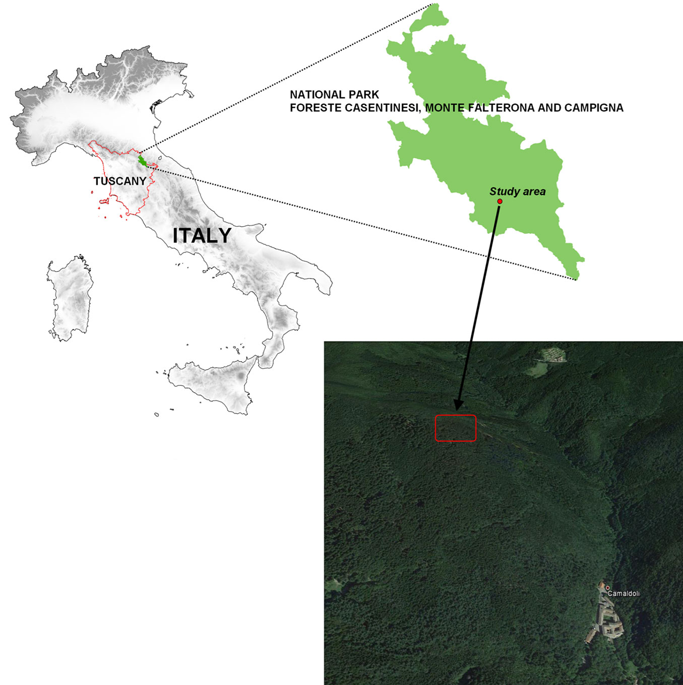
The TOOFES model was tested on an area located in the Foreste Casentinesi, Monte Falterona and Campigna National Park (Tuscany, Italy). The national park covers more than 36.000 ha in a mountainous region of the Apennines between Emilia-Romagna and Tuscany. Forests are extended over about 83% of the area and are mainly dominated by hornbeams, turkey oaks, sessile oaks and chestnut woods. Conifer stands (e.g., silver fir Abies alba Mill.) and artificial black pine forests also cover a significant area. The test area was located in the heart of the National Park close (1.1 km) to the Holy Hermitage of Camaldoli, a monastery founded in 1012 (Fig. 3). The forest is characterized by a 1-ha silver fir compartment. The study area was chosen for its representativeness at wider spatial scales, both regional and national. Silver fir forests in Italy are mainly artificial stands in the mountainous areas of the Apennines and Alps as well as on public property (73%), as in the case of the examined parcel. The input data for the case study are reported in Tab. 1.
Fig. 3 - Location of the study area (43° 47′ 58.39″ N, 11° 48′ 47.57″ E). Source: Google Earth®. Image: August 29, 2014. Last accessed: January 23, 2017.
Tab. 1 - Model input data for the case study area.
| Data | U.M. or code | Value | Source and/or notes |
|---|---|---|---|
| Age | years | 50 | Regional Forest Inventory and field survey |
| Surface | ha | 1 | Photointerpretation and field survey |
| Rotation period | years | Sensitivity analysis | - |
| Management | (1): high forest (2): coppice |
1 | Final felling: clear cut in accordance with Tuscany Region Forestry Law ([51]) |
| Thinning | (1): presence (0): absence |
Sensitivity analysis | - |
| Age of thinning | year | 30 | ISAFA ([28]); 26% of biomass removal was considered |
| Slope | % | 33 | Regional Forest Inventory |
| Distance from roads | m | 808 | Regional Forest Inventory |
| Fertility | (1): very low; (2): low; (3): medium; (4): high; (5): very high |
5 | Regional Forest Inventory |
| Volume | m3 ha-1 | Related to age and yield table |
ISAFA ([28]) |
| Diameter | cm | Related to age and yield table |
ISAFA ([28]) |
| Discount rate | % | Sensitivity analysis | - |
| Class of assortments | (a): first class (b): second class (c): third class |
Diameter: (a): <20cm (b): 20-40cm (c): >40cm |
Technical literature (⇒ http://www.rivistasherwood.it/tecniko-e-pratiko.html); survey by local experts |
| Price for each class of assortment | € m-3 | (a): 25 (b): 48 (c): 73 |
Technical literature (⇒ http://www.rivistasherwood.it/tecniko-e-pratiko.html); survey by local experts |
| Production costs | € m-3 | Calculated following Sacchelli et al. ([43]) | Dendrometric parameters were processed using TOOFES. No renovation costs are included (natural renovation is hypothesized - [51]) |
| Biomass Expansion Factor | - | 1.34 | Federici et al. ([17]) |
| Wood Basic Density | Dry weight tons m-3 | 0.38 | Federici et al. ([17]) |
| Root/shoot ratio | - | 0.28 | Federici et al. ([17]) |
| Carbon price | € t-1 | 7 | CMCC ([9]) |
| Biodiversity value | € ha-1 year-1 | 45 | Ten Brink et al. ([48]). WTP per person per year for woodland was calibrated on Tuscany residents |
| Land use at year 0 | See chapter “Model approach” |
7 7 5 7 × 7 7 6 6 |
Photointerpretation and field survey |
| Touristic recreational value | € ha-1 year-1 | 27 | Riccioli et al. ([40]) |
| Selected age for analysis of touristic recreational value | years | 100 | The age was set at 100 years, as suggested in Rose & Chapman ([42]) |
Results and discussion
The first parameters analyzed were the different ES values for the stand (VPS, VRS, VSS, VCS, VES). The evaluation relates the above output to different factors, i.e., silvicultural parameters (rotation period, presence/absence of thinning) and an economic parameter (discount rate - Fig. 4).
Fig. 4 - Variation in economic value (€, y-axis) with respect to rotation period (years, in x-axis), thinning intervention and discount rate. (a): absence of thinning, 2% discount rate; (b): absence of thinning, 4% discount rate; (c): thinning at year 30, 2% discount rate; (d): thinning at year 30, 4% discount rate.
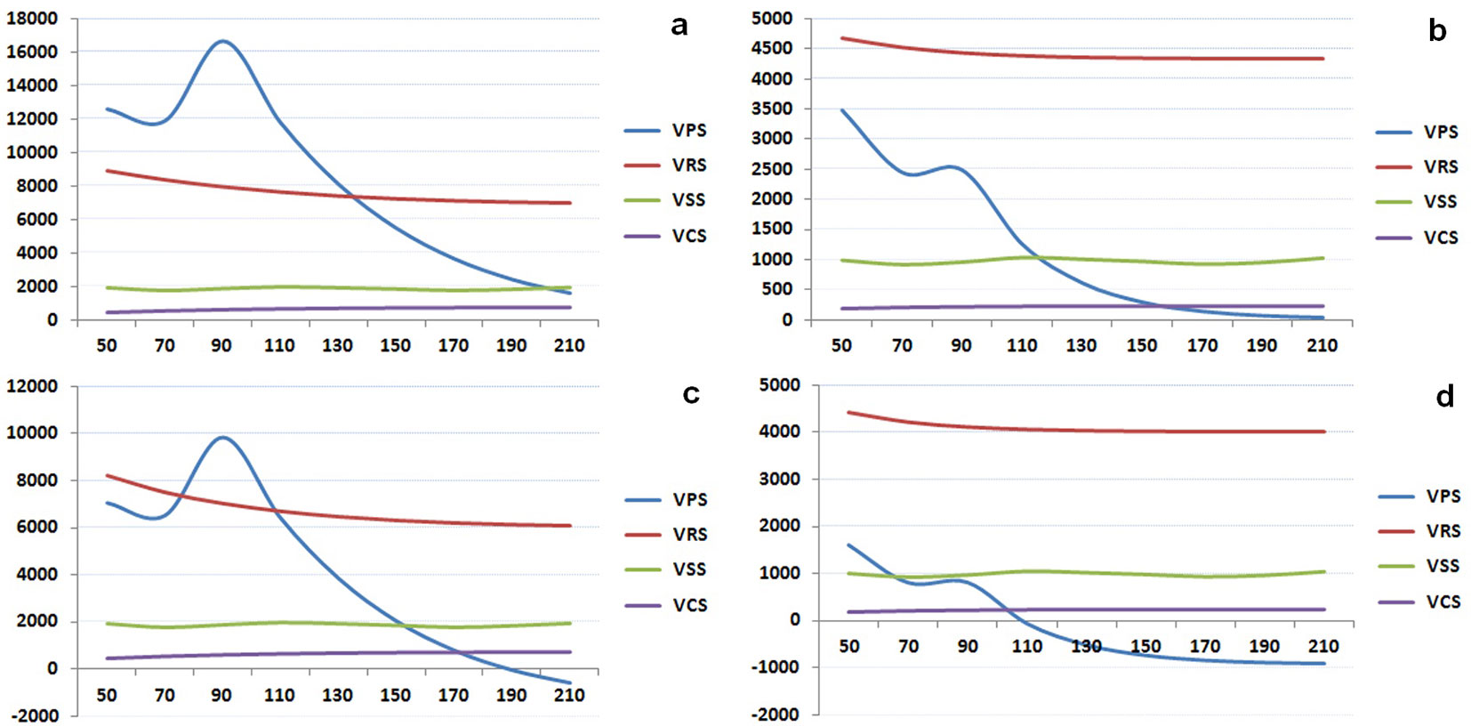
The increase in discount rate from 2% to 4% obviously led to poorer economic results for all V* typologies: 89% for VPS, 40% for VRS, 40% for VSS and 64% for VCS, with an average 57% decrease overall.
Sensitivity analyses based on rotation length show different trends for each ecosystem service. In general, for low discount rates (2%) the VPS peaks at around 90 years, and then decreases progressively. If the discount rate is increased to 4%, a shorter rotation appears to be the best option for improving the VPS. The characteristics of the study area confirm past experience in conifer stands of the Italian Apennines and Italy in general, where thinning often leads to negative stumpage values. In this case the stumpage value after thinning is lesser than zero and, as expected, the capitalized VPS with thinning is lower than the VPS without thinning. Due to the greater increase in annual volume for the early stand ages, the VRS tends to decrease as the rotation period increases. The VCS shows an opposite trend. This value is strictly related to certain tree dimensions (in particular the mean diameter). Higher rotation lengths lead to an increase in the economic value of cultural services. Thinning seems to be the best practice for improving the VCS. Thinning increases the VCS by about 3%, supporting assertions by Ribe ([39]) and Lupp et al. ([31]). Ribe ([39]) related the visual importance of forests to diameter, while Lupp et al. ([31]) suggest that although thinning has a positive effect on visual impact, this effect is very subtle in conifer stands.
VSS trends fluctuate instead; the value depends on the relative complexity of examined patterns and is based on land use as well as the age of close stands. It ranges from a minimum of 923 € to a maximum of 1949 € in the considered rotation period (50-210 years).
Among total values, the VPS appears to be the one that fluctuates the most with rotation length and discount rate (values from -904 € to 16.643 €). For low discount rates and shorter rotation ages, it is the most important component of the VES. Should the above parameters increase, it could also reaches negative values (Fig. 4c, Fig. 4d). The VRS is also somewhat important, with values ranging from 4.017 to 8.940 €. Lastly, VCS can vary from a minimum of 178 to a maximum of 739 €.
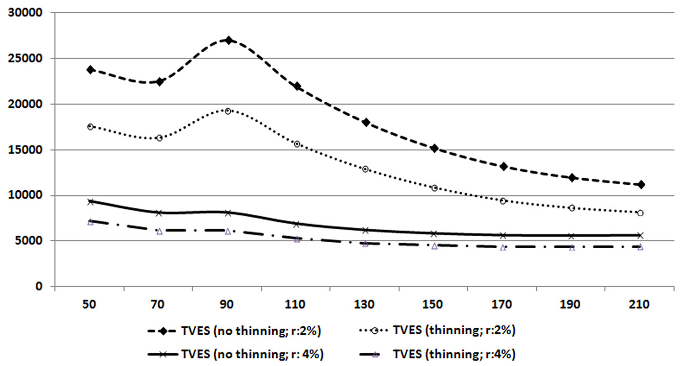
The VES ranges from 4.332 to 27.049 € (Fig. 5). The main factor affecting the VES is the discount rate, with an average 62% recorded decrease when the discount rate increases from 2% to 4%. Taking into account forest treatment, the presence of thinning reduces the VES by about 26%.
Fig. 5 - Variation in the economic value of ecosystem services (€, y-axis) with respect to rotation period (years, x-axis), thinning intervention and discount rate.
Another issue that can be investigated by TOOFES is the optimal rotation length to maximize the value of each forest function or, in other words:
- the provisioning services rotation period (PSRP): the rotation period for maximizing the VPS;
- regulating services rotation period (RSRP): the rotation period for maximizing the VRS;
- supporting services rotation period (SSRP): the rotation period for maximizing the VSS;
- cultural services rotation period (CSRP): the rotation period for maximizing the VCS;
- systemic rotation period (SRP): the rotation period for maximizing the VES.
Optimal ages are reported in Tab. 2, differentiated for ES, presence/absence of thinning, as well as discount rate (1-5%). The admissible rotation period Ω is set to 50-300 years. Tuscany Region Forestry Law (LR 48/2003) defines 70 years as the minimum rotation period for silver fir. In order to analyze a greater interval, 50 years was chosen as a valid lower limit for mature stands.
Tab. 2 - Optimal rotation periods and values of forest related to presence/absence of thinning and discount rate (r).
| Presence of thinning | Absence of thinning | ||||||||||
|---|---|---|---|---|---|---|---|---|---|---|---|
| r | 1% | 2% | 3% | 4% | 5% | r | 1% | 2% | 3% | 4% | 5% |
| PSRP | 88 | 88 | 88 | 50 | 50 | PSRP | 81 | 81 | 81 | 50 | 50 |
| VPS | 57899 | 17198 | 6491 | 3480 | 2028 | VPS | 39981 | 11645 | 4111 | 1597 | 798 |
| VRS | 14928 | 8009 | 5661 | 4685 | 3821 | VRS | 13176 | 7220 | 5201 | 4425 | 3648 |
| VSS | 3643 | 1851 | 1257 | 997 | 815 | VSS | 3665 | 1851 | 1252 | 997 | 815 |
| VCS | 1328 | 578 | 334 | 178 | 131 | VCS | 1309 | 574 | 334 | 182 | 134 |
| VES | 77797 | 27635 | 13744 | 9340 | 6796 | VES | 58131 | 21289 | 10898 | 7201 | 5395 |
| RSRP | 50 | 50 | 50 | 50 | 50 | RSRP | 50 | 50 | 50 | 50 | 50 |
| VPS | 33050 | 12584 | 6285 | 3480 | 2028 | VPS | 19706 | 7032 | 3228 | 1597 | 798 |
| VRS | 17390 | 8940 | 6110 | 4685 | 3821 | VRS | 15716 | 8216 | 5699 | 4425 | 3648 |
| VSS | 3719 | 1904 | 1299 | 997 | 815 | VSS | 3719 | 1904 | 1299 | 997 | 815 |
| VCS | 903 | 419 | 258 | 178 | 131 | VCS | 927 | 429 | 263 | 182 | 134 |
| VES | 55062 | 23847 | 13953 | 9340 | 6796 | VES | 40068 | 17581 | 10489 | 7201 | 5395 |
| SSRP | 54 | 110 | 110 | 110 | 110 | SSRP | 54 | 110 | 110 | 110 | 110 |
| VPS | 34703 | 11762 | 3708 | 1248 | 431 | VPS | 20880 | 6379 | 1317 | -60 | -393 |
| VRS | 17101 | 7651 | 5524 | 4395 | 3671 | VRS | 15306 | 6701 | 4990 | 4066 | 3458 |
| VSS | 3775 | 1949 | 1345 | 1041 | 857 | VSS | 3775 | 1949 | 1345 | 1041 | 857 |
| VCS | 958 | 631 | 355 | 227 | 157 | VCS | 985 | 653 | 366 | 233 | 160 |
| VES | 56537 | 21994 | 10932 | 6910 | 5115 | VES | 40945 | 15682 | 8018 | 5279 | 4082 |
| CSRP | 300 | 300 | 300 | 300 | 300 | CSRP | 300 | 300 | 300 | 300 | 300 |
| VPS | 5916 | 293 | 293 | 1 | 0 | VPS | 1496 | -1463 | -1221 | -921 | -692 |
| VRS | 10075 | 6900 | 6900 | 4344 | 3656 | VRS | 8351 | 5853 | 4812 | 4016 | 3443 |
| VSS | 3512 | 1832 | 1832 | 978 | 803 | VSS | 3512 | 1749 | 1266 | 978 | 803 |
| VCS | 1948 | 726 | 726 | 233 | 159 | VCS | 1999 | 653 | 391 | 240 | 162 |
| VES | 21451 | 9751 | 9751 | 5557 | 4618 | VES | 15358 | 6783 | 5247 | 4313 | 3717 |
| SRP | 88 | 88 | 51 | 50 | 50 | SRP | 81 | 81 | 81 | 50 | 50 |
| VPS | 57899 | 17198 | 6299 | 3480 | 2028 | VPS | 39981 | 11645 | 4111 | 1597 | 798 |
| VRS | 14928 | 8009 | 6094 | 4685 | 3821 | VRS | 13176 | 7220 | 5201 | 4425 | 3648 |
| VSS | 3643 | 1851 | 1304 | 997 | 815 | VSS | 3665 | 1851 | 1252 | 997 | 815 |
| VCS | 1328 | 578 | 261 | 178 | 131 | VCS | 1309 | 574 | 334 | 182 | 134 |
| VES | 77797 | 27635 | 13958 | 9340 | 6796 | VES | 58131 | 21289 | 10898 | 7201 | 5395 |
The PSRP is equal to 88 years and decreases to the minimum allowable value (50 years) as the discount rate increases from 3% to 4%. In the case of thinning, the trend is similar but with a lower rotation age (81 years). In general, increasing the discount rate not only decreases the VPS but also shortens the PSRP.
As explained above, RSRP is strictly dependent on the annual increase in volume. This means that the minimum rotation period is always the best option when trying to maximize regulating services.
The VSS improves for SSRP of 54 to 110 years, in both the absence and presence of thinning. The SSRP (110 years) maximizes VSS when the discount rate is equal to or greater than 2%. Maximum VCS are associated with a CSRP equal to the highest admissible age, as discussed earlier.
Due to the great importance of the VPS of the examined forest, the SRP tends to correspond to the PSRP for the whole range of sensitivity analyses. The only exception is in the absence of thinning and for a 3% discount rate, which yield an intermediate value of 51 years that is probably influenced by the economic importance of carbon sequestration.
Once the total value has been optimized, decision makers have a guideline for analyzing different types of forest management. ES trade-off analysis provides another useful output. In other words, the variation (reduction) in value of a specific ecosystem service resulting from the maximization of other values should be highlighted, as indicated in Fig. 6.
Fig. 6 - Trade-off analysis among ES functions. Reduction in the value of a specific function (columns) when the value of another function is maximized (rows).
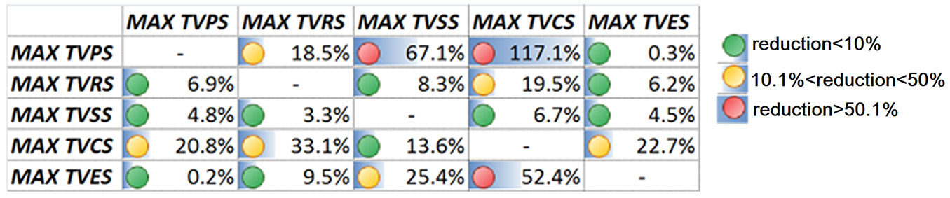
The greatest contrast among VPS, VSS and VCS is found in the case of VPS maximization. Production of traditional assortments is often in contrast with tourism-recreational functions and with preserving biodiversity. A similar trend is defined in maximizing the VES. The VRS decreases substantially when the VCS is improved (33% reduction). An interesting output is the low variability of the VPS, VRS, VCS and VES in the case of VSS maximization. In the case of this study it means that optimization of biodiversity shows a little conflict with other values.
Comparison of TOOFES with other tools for ES evaluation
A number of models and DSS for ES evaluation are described in the literature ([4]). In order to facilitate comparison between TOOFES and other available tools, the evaluative criteria proposed by Bagstad et al. ([4]) are briefly discussed. The criteria are: (i) quantification of output, nonmonetary and cultural perspectives, uncertainty evaluation; (ii) capacity of independent applications by users; (iii) level of development and documentation; (iv) scalability; (v) time requirements; (vi) generalizability; and (vii) affordability, insights, integration with existing environmental assessment.
- Quantification of output, nonmonetary and cultural perspectives, uncertainty evaluation. Outputs are calculated in quantitative terms. The monetary value of ES is the main output. Specific data (e.g., total cubic meters of assortments, total stored carbon, average relative richness and number of visits) can be selected by means of “summarize operation” on Processing sheet. Uncertainty can be analyzed using varying inputs (sensitivity analysis).
- Capacity of independent applications. The spreadsheet structure and open-source implementation facilitate the independent use of the model. TOOFES will be available on request by e-mailing the author.
- Level of development and documentation. TOOFES is fully documented for the analyzed ES. Additional ES functions can be included and documented in future versions.
- Scalability. Model outputs can be defined for different forest areas according to the size of the study area and available input data. TOOFES is designed for application at the stand scale, a scale considered suitable for decision support in operational forest management ([29]). The structure of the model is such that analyses can be undertaken at different scales, including large scales. This option is possible through the transformation of large-scale input data such as digital raster maps (forest information, roads, digital terrain models, etc.) into ASCII data. Said transformation can be completed in any classic Geographic Information System and allows this data to be input into a spreadsheet, thereby facilitating the optimization procedure.
- Time requirements. It does not take long to run the model once input data are available. In general, a few runs are necessary for the analysis of provisioning and regulating services. It can take much longer if field surveys are required to implement input data (usually for cultural services if the Benefit Transfer approach cannot be applied). The calculations in the optimization procedure take only a few minutes (for example, the SRP can be determined in about 2 minutes when using a calculator with a 3 GHz-processor and 8 GB of RAM). The computational time and CPU requirements increase for large-scale analyses.
- Generalizability. The high degree of customizability of input data facilitates the use of this tool.
- Affordability, insights, integration with existing environmental assessment. Model results can fit with established forest management and planning processes, taking into account normative prescriptions. For example, the optimization procedure can be carried out setting constraints such as the minimum rotation age admissible by local laws or additional quantitative parameters (minimum production of wood assortments or stored carbon, etc.). Forest management and silvicultural treatments can be calibrated in the DSS according to local peculiarities and practices. Thanks to its user-friendly output and graphical interface, TOOFES can be readily applied by decision makers.
Final remarks
This study implemented a Decision Support System (DSS) named TOOFES for quantifying economic value and trade-offs in forest ecosystem services (ES). The DSS enables the dynamic analysis and planning of forest functions throughout the forest life cycle. TOOFES is based on an open-source spreadsheet, allowing its ready and widespread application. The flexible structure allows for its application in different study areas and locations, and facilitates updating of ES and results. In this case study, TOOFES was applied to the analysis of homogenous stands at a small scale. The structure of the model also allows its application to large-scale evaluations, as already discussed. Other GIS-based models for quantifying ES (e.g., ARIES: ⇒ http://aries.inte gratedmodelling.org/; or InVEST: ⇒ http://www.naturalcapitalproject.org/invest/) could reduce the time required to analyse vaster, more complex areas. However, unlike other available tools, the structure of TOOFES is such that it can be used for more than just simple ES trade-off analysis. It allows the optimization of specific objective functions (e.g., maximizing the value of forest ES) by setting constraint parameters.
As in other modeling procedures, missing data in the analyzed area can create some problems in TOOFES. More general data can be used to substitute the missing one; however, the main problem lies in downscaling and the maximum standard error admitted in model outputs. For example, due to the scarcity of yield tables (norms) for uneven-aged stands at the national level, this first version of the model could be applied to even-aged forests, with more research needed for the analysis of uneven-aged stands. In TOOFES, monetary evaluations can consider the Net Present Value as well as the annual flow of ES, as in the majority of studies. However, output data focus on the capitalized value of the forest. When implementing Payments for Ecosystem Services (PES) schemes, in order to follow the dictates of economic valuation and appraisal in forestry, it seems more appropriate to determine the capitalized value rather than the NPV. Additional economic outputs may be investigated in future works. Tab. S1 (Supplementary material) reports other available outputs.
The main strength of the model is its ability to analyze complex systems. TOOFES improves upon the “static” evaluation presented in most scientific papers and DSS by taking into account the temporal variability of forest characteristics (e.g., volume and forest landscape). This can be useful in achieving the objective of sustainability in forest management. For example, in the framework of the 2030 Agenda for Sustainable Development, the identification of strategies for sustainable forest management (indicator 15.2.1) could facilitate the analysis of Sustainable Development Goal 15: “Protect, restore and promote sustainable use of terrestrial ecosystems, sustainably manage forests, combat desertification, and halt and reverse land degradation and halt biodiversity loss”.
Future analyses can introduce mixed-method valuation. Monetary calculations can be suitably integrated/substituted with non-monetary trade-offs based on multicriteria analysis and a combination of biophysical variables. This could lead to the development of alternative approaches to classical environmental economics. The lack of rivalry and excludability in public goods and services may lead to a difficult and controversial monetization of ES ([16]). This approach can possibly contribute to regional and national policies in that it allows the simultaneous quantification and planning of different ES in individual forested areas. Best management strategies can be developed taking into account the priorities and perceptions of different local stakeholders. Minimum levels of supplied ES can also be established and verified through scenario analysis. Guidelines for the emerging sector of Payment for Ecosystem Services could be established in line with the updated national normative framework (see Collegato Ambientale - [18]). In particular, the model could facilitate and improve methods for national ES accounting. Additional scenario analyses that take into account risk parameters as well as anthropogenic and natural damage assessment should be examined.
In conclusion, the proposed DSS with the suggested improvements could be an effective tool for the dynamic analysis and planning of forest ES.
References
CrossRef | Gscholar
Gscholar
CrossRef | Gscholar
Gscholar
Online | Gscholar
Gscholar
Gscholar
Gscholar
Authors’ Info
Authors’ Affiliation
Department of Agricultural, Food and Forest Systems Management, University of Florence, 18, p.le delle Cascine, I-50144, Florence (Italy)
Corresponding author
Paper Info
Citation
Sacchelli S (2018). A Decision Support System for trade-off analysis and dynamic evaluation of forest ecosystem services. iForest 11: 171-180. - doi: 10.3832/ifor2416-010
Academic Editor
Luca Salvati
Paper history
Received: Feb 23, 2017
Accepted: Nov 23, 2017
First online: Feb 19, 2018
Publication Date: Feb 28, 2018
Publication Time: 2.93 months
Copyright Information
© SISEF - The Italian Society of Silviculture and Forest Ecology 2018
Open Access
This article is distributed under the terms of the Creative Commons Attribution-Non Commercial 4.0 International (https://creativecommons.org/licenses/by-nc/4.0/), which permits unrestricted use, distribution, and reproduction in any medium, provided you give appropriate credit to the original author(s) and the source, provide a link to the Creative Commons license, and indicate if changes were made.

Web Metrics
Breakdown by View Type
Article Usage
Total Article Views: 51364
(from publication date up to now)
Breakdown by View Type
HTML Page Views: 40883
Abstract Page Views: 4541
PDF Downloads: 4687
Citation/Reference Downloads: 15
XML Downloads: 1238
Web Metrics
Days since publication: 3058
Overall contacts: 51364
Avg. contacts per week: 117.58
Article Citations
Article citations are based on data periodically collected from the Clarivate Web of Science web site
(last update: Mar 2025)
Total number of cites (since 2018): 9
Average cites per year: 1.13
Publication Metrics
by Dimensions ©
Articles citing this article
List of the papers citing this article based on CrossRef Cited-by.
Related Contents
iForest Similar Articles
Research Articles
Vascular plants diversity in short rotation coppices: a reliable source of ecosystem services or farmland dead loss?
vol. 13, pp. 345-350 (online: 17 August 2020)
Research Articles
The concept of green infrastructure and urban landscape planning: a challenge for urban forestry planning in Belgrade, Serbia
vol. 11, pp. 491-498 (online: 18 July 2018)
Research Articles
Green oriented urban development for urban ecosystem services provision in a medium sized city in southern Italy
vol. 7, pp. 385-395 (online: 19 May 2014)
Research Articles
Linking biomass production in short rotation coppice with soil protection and nature conservation
vol. 7, pp. 353-362 (online: 19 May 2014)
Research Articles
Communicating spatial planning decisions at the landscape and farm level with landscape visualization
vol. 7, pp. 434-442 (online: 19 May 2014)
Research Articles
Could cattle ranching and soybean cultivation be sustainable? A systematic review and a meta-analysis for the Amazon
vol. 14, pp. 285-298 (online: 08 June 2021)
Review Papers
Paying for water-related forest services: a survey on Italian payment mechanisms
vol. 5, pp. 210-215 (online: 12 August 2012)
Review Papers
Payment for forest environmental services: a meta-analysis of successful elements
vol. 6, pp. 141-149 (online: 08 April 2013)
Review Papers
Public participation: a need of forest planning
vol. 7, pp. 216-226 (online: 27 February 2014)
Review Papers
Green Infrastructure as a tool to support spatial planning in European urban regions
vol. 6, pp. 102-108 (online: 05 March 2013)
iForest Database Search
Search By Author
Search By Keyword
Google Scholar Search
Citing Articles
Search By Author
Search By Keywords
PubMed Search
Search By Author
Search By Keyword


