Climatic factors defining the height growth curve of forest species
iForest - Biogeosciences and Forestry, Volume 10, Issue 3, Pages 547-553 (2017)
doi: https://doi.org/10.3832/ifor2189-010
Published: May 05, 2017 - Copyright © 2017 SISEF
Research Articles
Abstract
The aim of this study was to modify several existing biological models by including several predictive variables that take into account the effect of climatic factors on tree height growth. Tree height was measured from 2007 to 2014 on 18 trees for each of the following species: Eucalyptus urophylla × Eucalyptus grandis, Parapiptadenia rigida, Peltophorum dubium, Mimosa scabrella and Schizolobium parahybae. Different existing nonlinear models were fitted to the observed data, and the best fitting models were selected. The inclusion of climatic variables into the selected models (mainly minimum temperature and rainfall) improved their predictions of tree height growth with age, and provided more accurate estimates than those obtained by traditional nonlinear models. Simulations were carried out to explore the variation of tree height growth under different minimum temperature and precipitation regimes. The effects of frost and rainfall variation on height growth curves and their consequences for forest management are discussed.
Keywords
Von Bertalanffy-Richards’ Model, Mean Minimum Temperature, Rainfall, Frost
Introduction
Tree height is an important variable used in tree volume estimation, as well as in making decisions on cultivation, planning and management of tree stands ([45]). The height of trees in plantations is related to the level of intra-specific interaction, planting arrangement ([2], [16]), soil characteristics and availability of nutrients ([25]), as well as the prevailing weather in the area ([7], [18]).
Tree height is commonly used in modeling the growth of trees ([46], [40], [15], [5], [30], [26], [4]). Regression models have been widely applied in several research areas. While regression linear models are easy to use, nonlinear models may be the most appropriate choice in many cases. A common example of the application of non-linear regression models in biology is their use in modeling tree growth curves by fitting nonlinear functions.
Biological growth models usually present the organism size or weight as the dependent variable, and the organism age as predictor, without taking into account climatic factors. In regions where trees are subjected to harsh winters with absolute minimum temperatures below zero and frost occurrence, tree species sensitive to cold may incur damages to apical buds. Damage caused by winter conditions can potentially limit the growth of the upper third of the trees. To date, these and other variations in the growth curve due to climatic factors are not explained by biological models in the literature.
Evidence of the importance of using climatic factors in forest modeling to explain the responses of tree species have been documented in several reports ([38], [27], [28], [39]). According to several authors ([12], [43], [35], [36]), the predictive power of empirical models used to describe growth data can be improved by the incorporation of indices which account for climatic factors.
In this study we tested the hypothesis that climatic factors, along with plant age, can be profitably used to define height growth curves of forest tree species. To this purpose, we modified several existing biological models by adding predictive variables that take into account the effect of climatic factors on tree height growth.
Material and methods
Data source
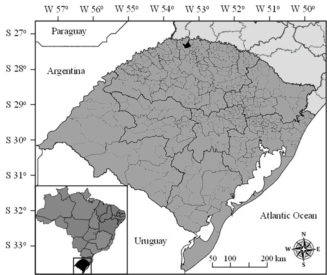
The study was conducted in the city of Frederico Westphalen, Rio Grande do Sul, Brazil, located at 27° 22′ S, 53° 25′ W at the altitude of 480 m a.s.l. (Fig. 1). The following tree species were used: Eucalyptus urophylla S.T. Blake × Eucalyptus grandis Hill ex Maiden, Mimosa scabrella Benth., Parapiptadenia rigida, Peltophorum dubium (Spr.) Taubert and Schizolobium parahybae (Vell.) Blake.
Fig. 1 - Geographical location of the experiment. The state of Rio Grande do Sul is highlighted in black on the bottom map, while the city of Frederico Westphalen is highlighted in black on the main map.
The experiment was established in September 2007, through the manual planting of seedlings after ploughing and harrowing the area. The experimental design was a randomized complete block design and the variables measured were the tree species, tree age and height, with three replicates for each treatment.
The determination of tree height began in March 2008, at the beginning of the autumn season, by selecting 18 trees of each species for the analysis. Since then, quarterly evaluations were carried out on the selected trees at the beginning of each season, until spring 2014. Tree height was measured from the ground level to the top leaf axils using a measuring tape until they reached 2.0 m, and using a Vertex III Hypsometer thereafter.
Height modeling
Seven non-linear models (Schumacher, von Bertalanffy-Richards, Clutter-Jones, Prodan, Mitscherlich, Gompertz, and Bailey with 4 parameters) were tested in order to estimate the tree height as a function of age, as described in Tab. S1 (Supplementary material).
Model performances were evaluated by the following criteria: coefficient of variation (CV, %), standard error (SE, m), graphic analysis of residuals (%), and the Pearson’s correlation coefficient between observed values and model predictions. For the estimation of nonlinear regression models, we used the nonlinear procedure “proc nlin” of the Statistical Analysis System (SAS®) software.
Comparison between model coefficients
When the same model has been selected for more than one species, the model coefficients were compared for their equality. To this purpose, we use the likelihood ratio test with accuracy given by chi-square (χ2) statistic ([31]). The method involves the addition of two independent variables, D1 and D2, in order to calculate the maximum likelihood estimates of the parameters under no restrictions in the parametric space (Ω) representing the complete model, and under restriction represented by ω in the reduced model.
The maximum likelihood ratio test (L) for large samples of size N was applied using the following formula ([29] - eqn. 1):
where σΩ2 is the estimate of the maximum likelihood of σ2 with no restriction on the parametric space, σϖ2 is the estimate of the maximum likelihood of σ2 with restrictions placed on H0, and N is the number of observations.
The complete model was adjusted under no restrictions in Ω, and the reduced model was adjusted with respect to restrictions defined in H0. When χ2calc ≥ χ2α at the significance level α, H0 was rejected.
Inclusion of climatic factors
After the selection of the models showing the best fitting for each species, we included climate factors as additional predictors into the model equations. Climatic data were obtained from the weather station of the Brazilian National Institute of Meteorology, located 1500 m away from the study site (27° 39′ S, 53° 43′ W). The following parameters were considered: mean temperature (Tmean), maximum (Tmax), minimum (Tmin), absolute minimum (Tminabs), absolute maximum (Tmaxabs); accumulated rainfall along the seasons (Prec); accumulated solar radiation along the season (Asr). The above climatic parameters were averaged over each season in the period 2008-2014.
The first step was to determine which of the climatic variables were most correlated with the dependent variable, i.e., tree height. The selection was undertaken using stepwise multiple regression techniques in SAS®.
The models obtained using the stepwise method were evaluated for the presence and magnitude of multicollinearity through the matrix condition number (ratio between the largest and smallest eigenvalues) and the variance inflation factors (VIFs). VIFs above 10 indicate a high degree of multicollinearity ([20]), due to the high correlation between independent variables in the model. This can result in an increased variance of the coefficients, thus compromising the final estimates. Therefore, variables showing high VIFs were excluded from the analysis. Multicollinearity was considered weak, moderate or severe, when the condition number was <100, between 100 and 1000, or >1000, respectively ([21]).
The meteorological variables selected by the stepwise method were considered as additional explanatory variables; nonlinear models selected for each species were re-fitted. New parameters (βn) were added to the models and the coefficients were re-estimated.
Results
Best fitting models
The fit statistics for each model tested for each tree species are shown in Tab. 1. The best-fitting models selected for each species were: von Bertalanffy-Richards for Eucalyptus urophylla × E. grandis, Parapiptadenia rigida and Peltophorum dubium; Clutter-Jones for Mimosa scabrella; Gompertz for Schizolobium parahybae.
Tab. 1 - Fit statistics and coefficients obtained by fitting seven nonlinear models to describe the height growth of five tree species. The models used (see also Tab. S1 in Supplementary material) were: (Sch) Schumacher; (vB-R) von Bertalanffy-Richards; (C-J) Clutter-Jones; (Pro) Prodan; (Mit) Mitscherlich; (Gom) Gompertz; (B4P) Bailey 4P. (CV): coefficient of variation; (SE): standard error.
| Species | Model | Coefficients | CV (%) |
SE (m) |
|||
|---|---|---|---|---|---|---|---|
β 0 |
β 1 |
β 2 |
β 3 |
||||
|
Parapiptadenia
rigida |
Sch | 9.9513 | -925.4 | - | - | 37.75 | 1.56 |
| VB-R | 43.7913 | 0.000053 | 0.8691 | - | 34.42 | 1.43 | |
| C-J | 533 | -1.2948 | 0.0653 | 2.8678 | 35.12 | 1.46 | |
| Pro | -14073.4 | 302.6 | 0.00657 | - | 33.38 | 1.38 | |
| Mit | 97.2811 | 0.9925 | 0.000025 | - | 36.63 | 1.52 | |
| Gom | 192.3 | 4.931 | 0.000185 | - | 32.56 | 1.35 | |
| B4P | 16.988 | 0.0652 | 0.4175 | 4.4619 | 36.13 | 1.50 | |
| Mimosa scabrella | Sch | 4.9364 | -201.5 | - | - | 24.67 | 0.72 |
| vB-R | 4.4936 | 0.00252 | 1.0117 | - | 24.3 | 0.71 | |
| C-J | 5.3578 | -0.0708 | -0.6795 | 502.4 | 17.78 | 0.52 | |
| Pro | 3044.3 | 58.5306 | 0.1833 | - | 24.27 | 0.71 | |
| Mit | 4.4816 | 1.0129 | 0.00255 | - | 24.29 | 0.71 | |
| Gom | 4.302 | 2.1256 | 0.00403 | - | 24.6 | 0.72 | |
| B4P | 4.8284 | 0.1434 | 0.4536 | 4.3258 | 24.34 | 0.71 | |
| Peltophorum dubium | Sch | 10.4082 | -1051.8 | - | - | 26.58 | 1.13 |
| vB-R | 42.0389 | 0.000055 | 0.8688 | - | 23.97 | 1.02 | |
| C-J | 52.7337 | -3.858 | -0.3189 | 4.9368 | 26.79 | 1.14 | |
| Pro | -10654.3 | 296.9 | 0.0164 | - | 23.63 | 1.00 | |
| Mit | 121.5000 | 0.9967 | 0.000023 | - | 23.76 | 1.01 | |
| Gom | 14.7824 | 2.701 | 0.000562 | - | 24.11 | 1.02 | |
| B4P | 14.3982 | 0.0318 | 0.506 | 3.4676 | 24.94 | 1.06 | |
| Eucalyptus urophylla × E. grandis |
Sch | 28.35 | -700 | - | - | 17.4 | 1.99 |
| vB-R | 26.1731 | 0.00078 | 1.3692 | - | 16.23 | 1.85 | |
| C-J | 69.1835 | -0.6129 | -0.2858 | 18.5375 | 25.04 | 2.86 | |
| Pro | 13238.9 | 50.1822 | 0.0246 | - | 16.24 | 1.86 | |
| Mit | 30.9423 | 1.0364 | 0.000489 | - | 16.23 | 1.85 | |
| Gom | 22.2104 | 3.0673 | 0.0015 | - | 16.57 | 1.89 | |
| B4P | 28.3361 | 0.00611 | 0.7443 | 2.1138 | 16.25 | 1.86 | |
| Schizolobium parahybae | Sch | 9.5564 | -987 | - | - | 34.21 | 1.13 |
| vB-R | 30.5062 | 0.000016 | 0.5416 | - | 37.68 | 1.25 | |
| C-J | 26.279 | -1.1519 | -0.0418 | 0.9824 | 45.93 | 1.52 | |
| Pro | -13475 | 296.4 | 0.0244 | - | 30.08 | 1.00 | |
| Mit | 166.1000 | 0.997 | 0.000017 | - | 29.9 | 0.99 | |
| Gom | 10.1216 | 2.5814 | 0.000793 | - | 30.15 | 1.00 | |
| B4P | 10.2222 | 0.0001 | 1.175 | 0.9438 | 31.61 | 1.05 | |
Comparison between model coefficients
Tab. 2 reports the results of the likelihood ratio test performed for the three species modeled using the same model (von Bertalanffy-Richards). Based on χ2 statistic, the H0 was rejected for the following combinations: (i) Eucalyptus urophylla × E. grandis × Parapiptadenia rigida (EU × PR); (ii) Eucalyptus urophylla × E. grandis × Peltophorum dubium (EU × PD). This demonstrated that the equations differed for at least one parameter, and therefore that the common equation (whose estimates are listed in ω) cannot be used. Contrastingly, for the combination PR × DP (Parapiptadenia rigida × Peltophorum dubium), the hypothesis of equality of model parameters in the two groups (complete model and reduced model) was not rejected, thus the coefficients chosen were those listed in ω.
Tab. 2 - Parameter estimation of the complete model (Ω) and reduced model (ω) for the species combinations Eucalyptus urophylla × E. grandis (EU), Parapiptadenia rigida (PR) and Peltophorum dubium (PD). (SQRR): sum of squares residual of the regression; (DFRR) number of degrees of freedom of the regression residuals; (N): sample size; (χ2calc.): calculated chi-square values; (DF): degrees of freedom (P): critical probability level.
| Parameters | Species combination | |||||
|---|---|---|---|---|---|---|
| EU × PR | EU × PD | PR × PD | ||||
| Ω | ω | Ω | ω | Ω | ω | |
β 0a |
26.1731 | - | 26.1731 | - | 43.7913 | - |
β 1a |
0.00078 | - | 0.00078 | - | 0.000053 | - |
β 2a |
1.3692 | - | 1.3692 | - | 0.8691 | - |
β 0b |
43.7913 | - | 42.0389 | - | 42.0389 | - |
β 1b |
0.000053 | - | 0.000055 | - | 0.000055 | - |
β 2b |
0.8691 | - | 0.8688 | - | 0.8688 | - |
β 0 |
- | 35.6397 | - | 16.2705 | - | 42.9151 |
β 1 |
- | 0.000176 | - | 0.000624 | - | 0.000054 |
β 2 |
- | 0.847 | - | 1.06 | - | 0.869 |
| SQRR | 1814.9 | 14865.4 | 1608.4 | 17700.1 | 1003.107 | 1003.9 |
| DFRR | 650 | 653 | 738 | 741 | 684 | 687 |
| N | 656 | 744 | 690 | |||
| χ2calc. | 1379.57 | 1784.35 | 0.55 | |||
| DF (χ2) | 3 | 3 | 3 | |||
| P (χ2v > χ2calc.) | 1.46 x 10⁻¹² | 1.88 x 10⁻¹² | 0.91 | |||
Estimating tree species’ height
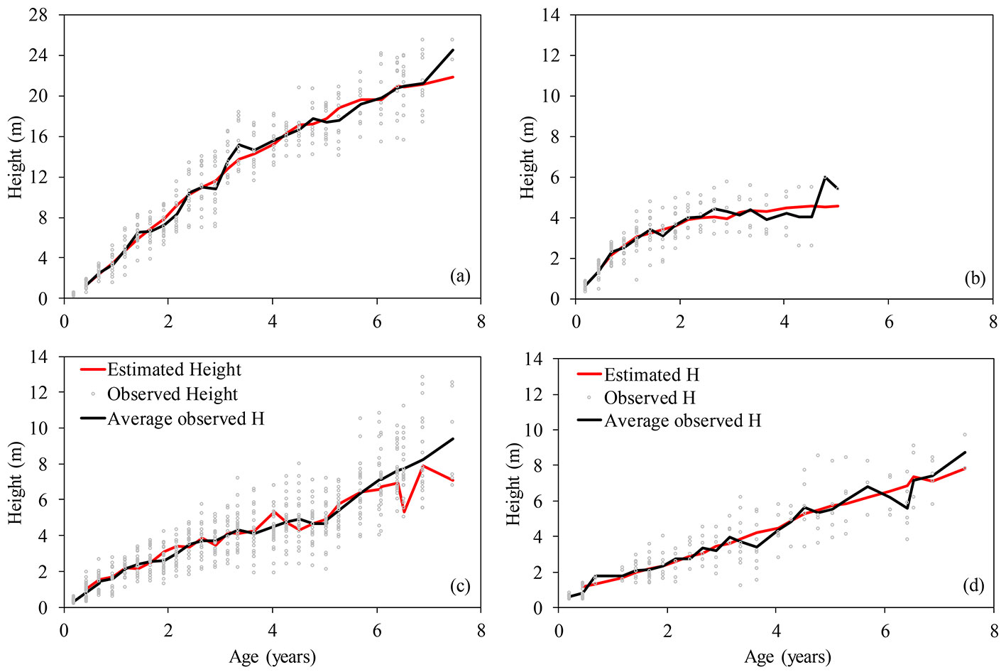
To assess the change in tree height with age for the species studied, we plotted the growth curves obtained by the use of the best fitting models described above (Fig. 2). The best relationship between the observed and predicted values was detected for Eucalyptus urophylla × E. grandis. For this species, the average observed height (black line in Fig. 2) significantly diverges from the height predicted by the model (red line), likely due to frost occurrence in several years that has lowered the growth of trees at the study site. Similar gaps between the observed and predicted height values could also be noticed for the other studied species (Fig. 2).
Fig. 2 - Height growth curve according to age for different forest tree species. Grey dots represents the observed tree height values, the black line is the average of the observed heights in each year of observation, while the red line represents the predicted tree height at different ages obtained by the best-fitting model for each tree species. (a) Eucalyptus urophylla × E. grandis; (b) Mimosa scabrella; (c) Parapiptadenia rigida and Peltophorum dubium; (d) Schizolobium parahybae.
Selection of climatic factors
The inclusion of climatic factors in the models described above aimed at bridging the gap between observed and predicted tree height growth, as tree growth does not only depend on age. The climate variables tested at the study site are shown in Tab. 3. A wide variation in several climatic parameters was observed over the years, as well as the irregularity of rainfall across years and the occurrence of absolute minimum temperature lower than zero.
Tab. 3 - Mean temperature (Tmean), maximum (Tmax), minimum (Tmin), absolute minimum (Tminabs), absolute maximum (Tmaxabs); accumulated rainfall (Prec) along the seasons; accumulated solar radiation (Asr) along the season. Data are means over each season for the period 2008-2014 (source: Brazilian National Institute of Meteorology).
| Years | Seasons | Climatic factors | ||||||
|---|---|---|---|---|---|---|---|---|
| Tmean (°C) |
Tmax (°C) |
Tmin (°C) |
Tmaxabs (°C) |
Tminabs (°C) |
Prec (mm) |
Asr (MJ m-2) |
||
| 2008 | Summer | 23.24 | 24.04 | 22.48 | 34.00 | 13.40 | 333.20 | 2034.08 |
| Autumn | 16.73 | 17.47 | 16.00 | 31.80 | -2.10 | 526.60 | 3245.71 | |
| Winter | 16.15 | 16.80 | 15.52 | 32.70 | 0.40 | 316.40 | 4396.92 | |
| Spring | 20.43 | 21.15 | 19.76 | 36.70 | 4.70 | 587.00 | 6309.70 | |
| 2009 | Summer | 23.32 | 24.10 | 22.57 | 35.10 | 12.50 | 293.20 | 8311.97 |
| Autumn | 18.12 | 18.92 | 17.34 | 33.80 | -0.60 | 359.00 | 9620.18 | |
| Winter | 15.03 | 15.65 | 14.44 | 31.30 | -2.70 | 671.60 | 10664.73 | |
| Spring | 21.19 | 21.86 | 20.56 | 35.90 | 5.60 | 730.00 | 12389.98 | |
| 2010 | Summer | 24.07 | 24.80 | 23.39 | 35.70 | 13.60 | 478.80 | 14306.95 |
| Autumn | 17.10 | 17.69 | 16.54 | 31.50 | 3.00 | 706.80 | 15377.76 | |
| Winter | 15.56 | 16.17 | 14.95 | 31.30 | -1.80 | 312.60 | 16509.36 | |
| Spring | 19.68 | 20.44 | 18.96 | 33.10 | 6.70 | 589.80 | 18393.55 | |
| 2011 | Summer | 23.39 | 24.11 | 22.73 | 33.36 | 13.10 | 464.20 | 20293.52 |
| Autumn | 17.32 | 17.99 | 16.68 | 31.10 | 2.40 | 425.80 | 21481.79 | |
| Winter | 14.97 | 15.56 | 14.41 | 31.70 | -2.60 | 892.80 | 22505.30 | |
| Spring | 20.67 | 21.47 | 19.89 | 34.70 | 8.50 | 436.80 | 24599.31 | |
| 2012 | Summer | 24.57 | 25.47 | 23.71 | 37.00 | 13.30 | 252.40 | 26781.67 |
| Autumn | 17.17 | 17.91 | 16.46 | 32.00 | -2.20 | 295.80 | 28021.24 | |
| Winter | 17.16 | 17.82 | 16.51 | 35.70 | 0.90 | 328.40 | 29391.31 | |
| Spring | 21.57 | 22.31 | 20.85 | 34.80 | 2.30 | 598.00 | 31482.57 | |
| 2013 | Summer | 22.39 | 23.10 | 21.71 | 35.90 | 11.50 | 573.60 | 33479.46 |
| Autumn | 17.12 | 17.81 | 16.46 | 29.90 | 3.00 | 435.60 | 34911.44 | |
| Winter | 14.72 | 15.38 | 14.08 | 32.90 | -1.80 | 520.60 | 36222.07 | |
| Spring | 20.78 | 21.50 | 20.10 | 34.10 | 5.60 | 510.80 | 38423.17 | |
| 2014 | Summer | 23.89 | 24.66 | 23.14 | 36.70 | 12.30 | 556.80 | 40636.56 |
| Autumn | 17.42 | 18.03 | 16.85 | 32.00 | 3.00 | 710.40 | 41978.62 | |
| Winter | 16.46 | 17.07 | 15.87 | 32.60 | 1.10 | 707.60 | 43298.17 | |
| Spring | 22.05 | 22.75 | 21.39 | 35.80 | 9.30 | 659.80 | 45403.82 | |
The climatic variables selected by the stepwise regression analysis were: Asr, Tmin and Prec for the Eucalyptus urophylla × E. grandis, Parapiptadenia rigida e Peltophorum dubium; Asr, Tmin, Prec and Tmean for Mimosa scabrella; Asr, Tminabs and Prec for Schizolobium parahybae. The very high correlation observed between independent variables indicates the presence of multicollinearity, as reported by Neter & Wasserman ([24]) and Sanquetta et al. ([33]). In this study, we used VIF = 10 as threshold for multicollinearity detection ([20]). The variables with high VIFs were age (A) and Asr; therefore Asr was excluded from the model. Its exclusion led to VIFs < 10, thus multicollinearity was considered weak by the selection methods.
Final models
After the inclusion of climate variables, the best nonlinear models formerly selected were re-fitted and the parameters were tested for their significance by t-tests. Tab. S2 in Supplementary material reports the final models after the inclusion of the climatic parameters and the species used in each model.
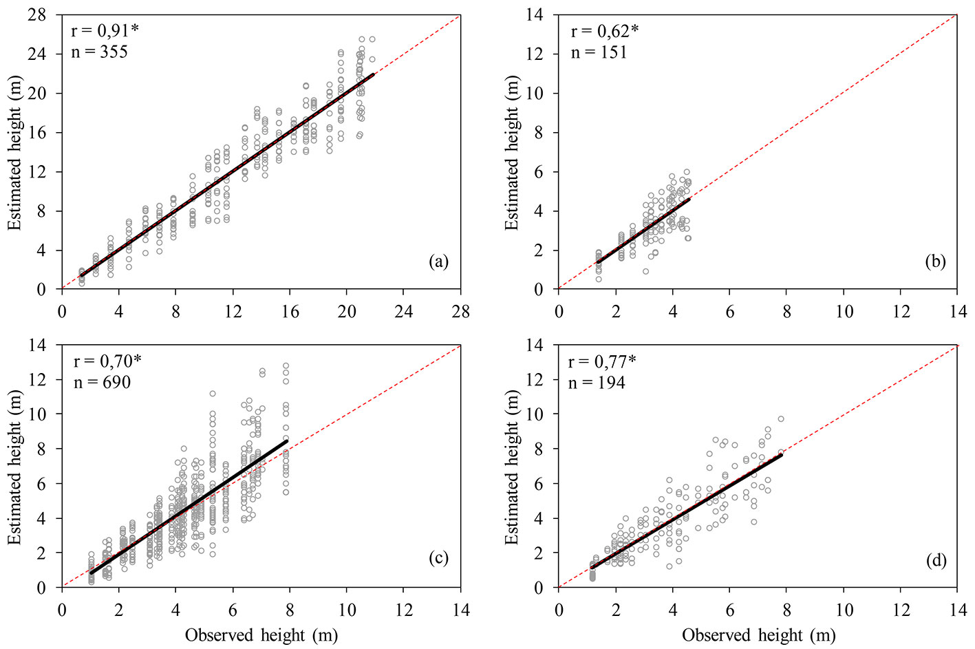
The adjusted coefficients for each final model are reported in Tab. 4. It is worth to notice that the inclusion of climatic parameters into the final models fairly reduced the gaps between the observed and predicted values of tree height growth (Fig. 3, Fig. 4). The residual analyses of these relationships are presented in Fig. S1 (Supplementary material) for each species.
Tab. 4 - Fit statistics and coefficients obtained by adjusting four nonlinear models based on climatic factors and tree age, to describe the height growth of different tree species. (CV): coefficient of variation; (SE): standard error.
| Species | Coefficients | CV (%) | SE (m) | |||||
|---|---|---|---|---|---|---|---|---|
β 0 |
β 1 |
β 2 |
β 3 |
β 4 |
β 5 |
|||
| Eucalyptus urophylla × E. grandis | 0.0109 | 0.1028 | 17.8813 | 0.0008 | 1.3824 | - | 16.61 | 0.58 |
| Mimosa scabrella | 0.0431 | 0.0871 | 7.1046 | -1.663 | -0.1112 | 0.7324 | 25.74 | 0.75 |
| Parapiptadenia rigida, Peltophorum dubium | 0.2192 | 10.5684 | 0.000023 | 0.6399 | - | - | 31.17 | 1.31 |
| Schizolobium parahybae | -0.0424 | 1.0002 | 15.0384 | 2.579 | -0.0007 | - | 31.60 | 1.05 |
Fig. 3 - Height growth curve according to age and climatic factors of different forest tree species. Grey dots represents the observed tree height values, the black line is the average of the observed heights in each year of observation, while the red line represents the predicted tree height at different ages obtained after the inclusion of climatic parameters in the models for each tree species. (a) Eucalyptus urophylla × E. grandis; (b) Mimosa scabrella; (c) Parapiptadenia rigida and Peltophorum dubium; (d) Schizolobium parahybae.
Fig. 4 - Relationship between estimated and observed height after the inclusion of climatic variables into tree height models: (a) Eucalyptus urophylla × E. grandis; (b) Mimosa scabrella; (c) Parapiptadenia rigida and Peltophorum dubium; (d) Schizolobium parahybae.
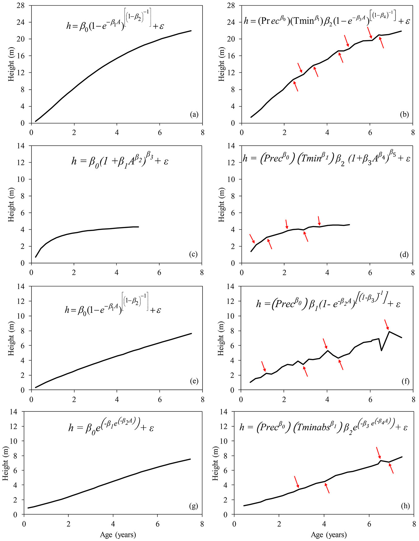
A comparison between by the traditional biological models and the final models including tree age and climatic factors as predictors is displayed in Fig. 5.
Fig. 5 - Variation in height growth curves before (left column: a, c, e, g) and after (right column: b, d, f, h) the inclusion of climatic factors in the traditional best-fitting models. The main differences between growth curves are indicated by red arrows. (a, b): Eucalyptus urophylla × Eucalyptus grandis; (c, d): Mimosa scabrella; (e, f): Parapiptadenia rigida and Peltophorum dubium; (g, h): Schizolobium parahybae.
Discussion
In this study, the non-linear regression models selected for estimating the height growth of each tree species considered seem biologically meaningful, and their fit statistics were satisfactory. In general, the von Bertalanffy-Richards model showed the best fit in most cases. Several authors have attributed the good performances of this model to its capacity to adequately describe the ecological/biological processes underlying tree growth ([44], [32], [4]).
The inclusion of climatic variables into the height growth models (Fig. 3) allowed to obtain more accurate estimates of tree height growth with age, as compared with those obtained using curves based on traditional nonlinear models. The standard error of the models was satisfactory and the coefficient of variation was acceptable (Tab. 4). In addition, the good consistency between observed and estimated values for all species in the models was detected by correlation analysis (Fig. 4).
It can be noticed that the minimum temperature and the accumulated rainfall over the seasons were the climatic parameters included in almost all the final models, and were therefore considered as the factors most affecting tree growth. The modifications of the growth curves after the inclusion of climatic parameters in the best fitting models are shown in Fig. 5. At many points along the curve, variations were observed in tree height (Fig. 5b, Fig. 5d, Fig. 5f and Fig. 5h) that were not identified using the traditional nonlinear models (Fig. 5a, Fig. 5c, Fig. 5e and Fig. 5g).
The impact of low temperatures on tree growth may vary depending on the species sensitivity, tree age, type of plant structure or organ, intensity of the minimum temperature and the occurrence and frequency of frost. This may result in the reduction of tree growth rate or biomass loss of the stem apex and leaves. Hendrickson et al. ([11]) found that minimum temperatures from 1 to 3 °C reduce the growth rate of Vitis vinifera by 34-63%. Gatti et al. ([8]) showed that low temperatures affect the photosynthetic rate of Euterpe edulis. Wang et al. ([42]) found that the occurrence of frost caused 31.3% defoliation of exposed shoots of Kandelia ovata. Augspurger ([3]) found that the death of branches reduced the canopy percentage, contributed to early senescence and reduced growth, and led to the death of Aesculus glabra yolks. Other studies showed that the occurrence of frost affects plant organs and their growth ([37], [19]), survival ([22]), reproduction ([14]) and demographic distribution ([13]). Freezing of extracellular solutions determines the senescence of leaves and stems, resulting in an imbalance between the chemical potential of intra and extra-cellular water. This leads to the water transfer outwards that causes cellular dehydration, decreased cell turgor, solute accumulation and rupture of the plasma membrane ([10]).
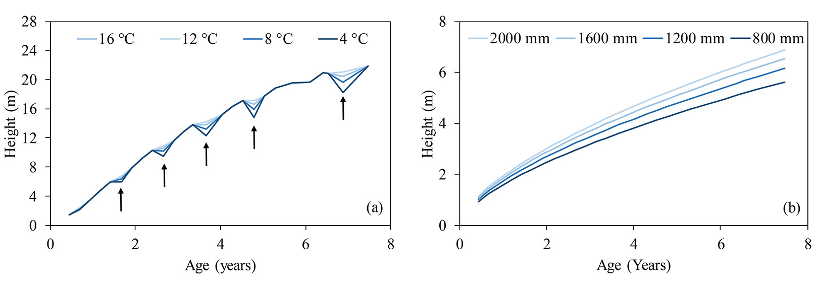
In this study we performed a simulation to explore the influence of different levels of minimum temperature occurring in winter and different annual rainfall regimes, on the height growth of the tree species studied, based on the model obtained (Fig. 6). The results confirmed that higher rainfall regimes have a positive impact on tree growth. This is consistent with the findings of Sanquetta et al. ([33]), who observed that the growth of Acacia mearnsii depends of available water content in the soil. Morales et al. ([23]) found high correlations between precipitation and the growth of Juglans australis, Alnus acuminata, Prosopis ferox and Polylepis tarapacana. Dünisch et al. ([6]) and Grogan & Schulze ([9]) obtained similar results with Swietenia macrophylla. Allen & Albaugh ([1]) reported that low water availability and extreme temperatures negatively affect the leaf area and the interception and use of solar radiation in Pinus taeda, influencing their overall growth.
Fig. 6 - Simulating height growth with age in Eucalyptus urophylla × E. grandis at different minimum temperatures (a), using the model h = (Precβ0) (Tmin β1) β2(1- e -β3A)1/(1-β4) + ε; Parapiptadenia rigida and Peltophorum dubium at different annual rainfall (b), using the model h = (Precβ0) β1(1-e -β2A)1/(1-β3) + ε. Black arrows represent the damage due to frosts in winter.
The water availability in the soil directly affects the transpiration rate, stomatal conductance, and photosynthesis ([34]), because the opening and closing of stomata are controlled by soil water potential. The absence of water stress allows increased internal CO2 concentration in the leaves due to greater stomatal conductance, increasing the photosynthetic rate ([17], [41]). These studies are in agreement with the results obtained in this study and with the climatic variables selected in the proposed models. The fact that the traditional nonlinear regression approach lead to a loss of path invariance can be considered, but the proposed models provide satisfactory estimates of the height of tree species, use easily obtainable input variables and are easily applicable in several forestry studies and practical situations.
Conclusions
Our results showed that the von Bertalanffy-Richards, Clutter-Jones and Gompertz models are more flexible in representing the growth of Eucalyptus urophylla x Eucalyptus grandis, Parapiptadenia rigida, Peltophorum dubium, Mimosa scabrella and Schizolobium parahybae.
The inclusion of climatic factors into such models improved their prediction of tree height growth with age. More accurate estimates were especially obtained by including minimum temperature and rainfall. Using the developed models, tree species growth can be simulated by changing weather conditions, thus providing useful information for the achievement of adequate forest management.
Acknowledgements
The authors acknowledge the National Council for Scientific and Technological Development (CNPq - Brazil) and the Coordination for the Improvement of Higher Education Personnel (CAPES - Brazil) for their financial support.
References
Gscholar
Gscholar
CrossRef | Gscholar
Authors’ Info
Authors’ Affiliation
Braulio Otomar Caron
Elder Eloy
Velci Queiróz De Souza
Felipe Schwerz
John Robert Stolzle
Federal University of Santa Maria, Frederico Westphalen Campus, Graduate Program in Agronomy - Agriculture and Environment. Linha Sete de Setembro n/a, Highway 386 km 40, CEP 98400-000, Frederico Westphalen, Rio Grande do Sul State (Brazil)
Federal University of Paraná, Graduate Program in Forest Engineering. Av. Pref. Lothário Meissner, 900, Jardim Bot’nico, Campus III, CEP 80210-160, Curitiba, Paraná (Brazil)
Corresponding author
Paper Info
Citation
Elli EF, Caron BO, Behling A, Eloy E, Queiróz De Souza V, Schwerz F, Stolzle JR (2017). Climatic factors defining the height growth curve of forest species. iForest 10: 547-553. - doi: 10.3832/ifor2189-010
Academic Editor
Giustino Tonon
Paper history
Received: Aug 03, 2016
Accepted: Feb 19, 2017
First online: May 05, 2017
Publication Date: Jun 30, 2017
Publication Time: 2.50 months
Copyright Information
© SISEF - The Italian Society of Silviculture and Forest Ecology 2017
Open Access
This article is distributed under the terms of the Creative Commons Attribution-Non Commercial 4.0 International (https://creativecommons.org/licenses/by-nc/4.0/), which permits unrestricted use, distribution, and reproduction in any medium, provided you give appropriate credit to the original author(s) and the source, provide a link to the Creative Commons license, and indicate if changes were made.
Web Metrics
Breakdown by View Type
Article Usage
Total Article Views: 53387
(from publication date up to now)
Breakdown by View Type
HTML Page Views: 43509
Abstract Page Views: 4312
PDF Downloads: 4070
Citation/Reference Downloads: 29
XML Downloads: 1467
Web Metrics
Days since publication: 3282
Overall contacts: 53387
Avg. contacts per week: 113.87
Article Citations
Article citations are based on data periodically collected from the Clarivate Web of Science web site
(last update: Mar 2025)
Total number of cites (since 2017): 15
Average cites per year: 1.67
Publication Metrics
by Dimensions ©
Articles citing this article
List of the papers citing this article based on CrossRef Cited-by.
Related Contents
iForest Similar Articles
Research Articles
Relationship between frost hardiness of adults and seedlings of different tree species
vol. 7, pp. 282-288 (online: 01 April 2014)
Research Articles
Frost damage to eucalypts in a short-rotation forestry trial in Cumbria (England)
vol. 7, pp. 156-161 (online: 23 January 2014)
Research Articles
Coping with spring frost-effects on polyamine metabolism of Scots pine seedlings
vol. 10, pp. 227-236 (online: 27 January 2017)
Review Papers
Integration of forest mapping and inventory to support forest management
vol. 3, pp. 59-64 (online: 17 May 2010)
Commentaries & Perspectives
Benefits of a strategic national forest inventory to science and society: the USDA Forest Service Forest Inventory and Analysis program
vol. 1, pp. 81-85 (online: 28 February 2008)
Research Articles
Simplified methods to inventory the current annual increment of forest standing volume
vol. 5, pp. 276-282 (online: 17 December 2012)
Research Articles
Frost hardening in seedlings of four provenances of Norway spruce in response to simulated autumn conditions with decreasing and fluctuating temperatures
vol. 19, pp. 141-148 (online: 19 April 2026)
Research Articles
Using self-organizing maps in the visualization and analysis of forest inventory
vol. 5, pp. 216-223 (online: 02 October 2012)
Research Articles
Estimation of stand crown cover using a generalized crown diameter model: application for the analysis of Portuguese cork oak stands stocking evolution
vol. 9, pp. 437-444 (online: 02 December 2015)
Research Articles
Nonlinear mixed model approaches to estimating merchantable bole volume for Pinus occidentalis
vol. 5, pp. 247-254 (online: 24 October 2012)
iForest Database Search
Search By Author
Search By Keyword
Google Scholar Search
Citing Articles
Search By Author
Search By Keywords
PubMed Search
Search By Author
Search By Keyword

