Disentangling the effects of age and global change on Douglas fir growth
iForest - Biogeosciences and Forestry, Volume 12, Issue 3, Pages 246-253 (2019)
doi: https://doi.org/10.3832/ifor2620-012
Published: May 03, 2019 - Copyright © 2019 SISEF
Research Articles
Abstract
Recent changes commonly observed in forests growth could be the result of a combination of different climatic and non-climatic factors, such as rising atmospheric [CO2], temperature changes, atmospheric N deposition and drought stress. These effects are difficult to assess, however, due to the superimposition of age-related changes. After removing age effects through a novel approach, this study quantifies the effects on tree growth of global change, and assesses the relationship with individual environmental drivers and their relative importance. Generalized Additive Mixed Models (GAMMs) were applied to decouple the non-linear effects of age and co-occurring environmental changes on basal area increments (BAI) series, as derived from tree rings in a Pseudotsuga menziesii stand chronosequence of four different age classes (65-, 80-, 100- and 120-year-old). The model could explain about 57% of the overall variation in BAI as a function of age and a selected set of predictors, including water availability in the current summer and at the end of previous growing season; together with age, winter-spring mean temperature was found to be the most important predictor. After accounting for age-related effects, a significant decrease in BAI was observed in Douglas fir over the last decades. No significant impact of atmospheric [CO2] and atmospheric N deposition were detected.
Keywords
Pseudotsuga menziesii, Basal Area Increments, Long-term Trends, Global Change, GAMM, Chronosequence
Introduction
Over recent decades, significant changes in forest growth have been observed, particularly in Europe, which have been interpreted as a result of the ongoing global change ([48]). However, the main drivers and functional basis of this trend have not been ascertained. The potential effect of atmospheric CO2 fertilisation during the Antrophocene is one of the most widely discussed explanations, based on the expected stimulation in photosynthetic rates at plant and ecosystem scale, with a positive effect on net primary productivity and growth. Only few experiments, however, have gathered suitable evidence to test this hypothesis ([2]), the majority of which did not find a clear relationship between elevated CO2 and growth enhancement ([23]). Other studies have reported such a positive link, although stressing the importance of concomitant related factors, for example disturbance history or an increasing length of the vegetative period ([28]). Indeed, interactions with other environmental variables such as atmospheric N deposition ([25]) are expected to play a determinant role especially in resource-limited environments. Moreover, a parallel increase in transpiration rates as a result of increasing temperatures could negate this positive effect, in particular in drought-prone areas ([18]). There is therefore a pressing need to understand which key drivers have been affecting forest growth rates, and quantify the magnitude of their effects. Even in the absence of controlled experiments, the analysis of long-term trends in tree growth can help elucidate the role of changes in different environmental factors, since the growth pattern of a tree is the result of surrounding conditions, as well as ontogenetic processes ([4]). Tree-ring widths (TRW) area direct measure of stem increments, hence the inspection of their time series provides a reliable and datable source of data that can be used to investigate high and low-frequency variability in forest growth trends. In order to highlight the environmental-related signals enclosed in tree-ring series, however, the superimposed age-(or size-) related signal must be first removed. An age-size related decline in TRW is generally observed with increasing age, due not only to geometrical constraints but also to hydraulic limitations related to tree height. In response to the increased hydraulic resistance of longer stems and branches and to the increased gravitational potential opposing the ascent of water, trees show a progressive reduction in stomatal conductance at old age and tend to reduce photosynthesis and growth ([30]). Basal area increments (BAI), on the contrary, generally display an increase with age, followed by a gradual stabilization. Canonical procedures applied in dendrochronological studies remove this age-related biological trend through the application of de-trending techniques, such as spline or negative exponential fitting ([33]). However, a consequence of this correction is the removal of low-frequency signals associated to tree-ring series ([12]). Preserving low-frequency variations is of fundamental importance if the objective of the analysis is to investigate long-term trends ([15]). In this study, Generalised Additive Mixed Models (GAMMs) were used as a tool to detect and separate the effect of different variables, both biological (i.e., age- or size-related) and environmental, on tree-ring trends in a Douglas fir (Pseudotsuga menziesii (Mirb.) Franco) chronosequence. This non-linear regression technique is a ceteris paribus form of analysis, looking at the effects of a single factor while keeping remaining factors constant ([37]). Tree age-size effects can be then considered as a simple additive variable, making it possible to disentangle the superimposed effects of other environmental covariates ([9]). Therefore, such a model can provide an alternative to traditional de-trending procedures, with the advantage of retaining low frequency variability in the time series. In addition, GAMMs preserve the non-linearity of the relationship between the response and the explanatory variables, in contrast with the assumption of linearity commonly made in dendroecological studies.
The aim of the present study is therefore to understand if Douglas fir has been affected by the changing environmental pressure in a long-term perspective, looking at which variable or combination of variables has driven any observed changes in growth rates.
Materials and methods
Study area
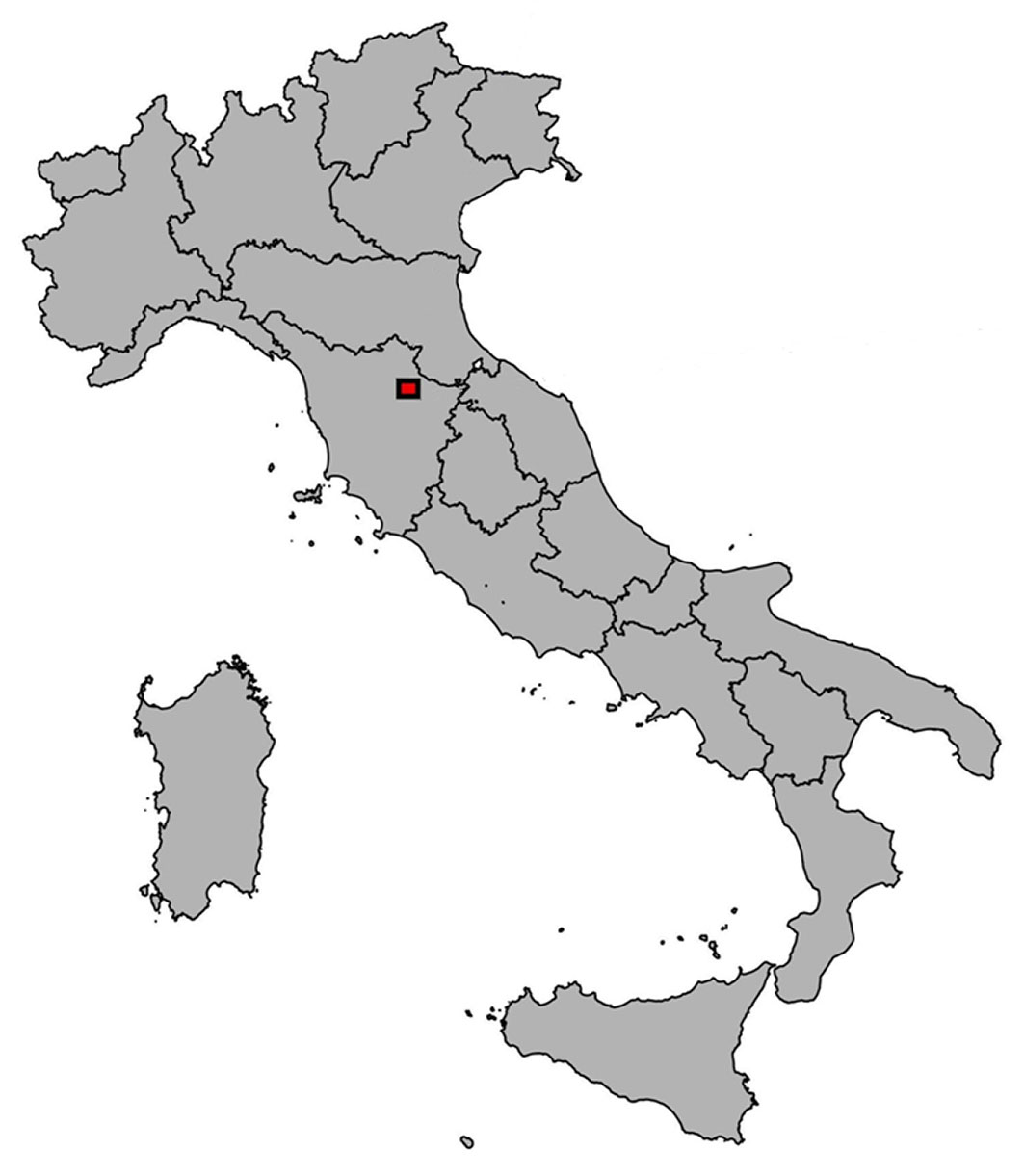
This study was performed in a Douglas fir plantation located in the Vallombrosa Forest, in the Apennine mountain range near Florence, Italy (43° 43′ 59.6″ N, 11° 33′ 16.9″ E - Fig. 1). The region has a Mediterranean climate without significant summer droughts; mean annual precipitation is approximately 1400 mm, of which only about 5% occur in summer months (72.48 mm). Mean annual temperature is 9.8 °C. The soils, derived from the Macigno del Chianti sandstone series, vary between Humic Dystrudept and Typic Humudept ([38]) in the younger and older stands, respectively, indicating similar soil conditions at the site. Douglas fir is a non-indigenous evergreen species which was imported from the Pacific Coast of the United States during the last decades of the 19th century; it was chosen for the present study because of its high economic importance. The sampled areas are part of the experimental permanent plot network managed by CREA Research Centre for Forestry and Wood (Arezzo, Italy), and include the oldest experimental plots established in Italy at the beginning of the 20th century ([32]). A chronosequence of plots was selected for the study; a chronosequence is here defined as a set of even-aged stands growing under the same environmental conditions and differing only for their age ([43]). The chronosequence approach made it possible to disentangle the effects of environmental changes from co-occurring changes in age and size. By comparing rings formed on the same calendar year (i.e., under identical environmental conditions) by trees of different age along the chronosequence, the approach makes it possible to highlight the real effect of age. On the other hand, considering rings formed at the same cambial age but in different calendar years, it is possible to isolate the true effect of varying environmental conditions.
Fig. 1 - Location of the study site (red square).
The chronosequence comprises four different age classes (65, 80, 100 and 120 years), covering the longest temporal interval that can be achieved in Italy for this species. The mean characteristics of the four age classes are summarized in Tab. 1. Seven plots were sampled that were consistent for management, aspect and elevation. Two plots were selected for each age class, in order to ensure replication; however this was not possible for the oldest class, as only one stand of this age was present in the area. In all plots, only dominant trees were chosen for the analysis, in order to avoid competition effects; repeated forest surveys on the same plots ensured the permanence of their dominant status at least for the last 40 years, as confirmed by an analysis of the Daniels’ competition index ([13] - see Fig. S1 in Supplementary material), independently of the management regime adopted (Fig. S2). Thinnings at the site are mainly from below, removing suppressed or intermediate trees which compete little with dominant trees. The use of survey data makes it possible to avoid potential sampling biases which occur when the currently largest-diameter trees are wrongly considered to have always been in the dominant class ([11]).
Tab. 1 - Mean characteristics of plots in the the Vallombrosa Douglas fir chronosequence. Mean ± standard error.
| Variable | Age-class | ||||||
|---|---|---|---|---|---|---|---|
| 120 | 100 | 80 | 65 | ||||
| Plot (code) | 1 | 2 | 3 | 4 | 5 | 6 | 7 |
| Age (yrs) | 117 ± 0.7 | 95 ± 0.7 | 94 ± 1.6 | 82 ± 0.4 | 81 ± 0.9 | 64 ± 0.8 | 62 ± 0.6 |
| Distance to the pith (cm) | 1.9 ± 0.8 | 2.4 ± 0.9 | 4.0 ± 1.3 | 1.7 ± 0.5 | 1.2 ± 0.3 | 2.1 ± 0.7 | 1.7 ± 0.6 |
| Years to the pith (rings) | 3.4 ± 1.3 | 3.6 ± 0.9 | 5.8 ± 1.4 | 2.6 ± 0.4 | 1.8 ± 0.4 | 2.8 ± 0.7 | 2.8 ± 0.9 |
| Elevation (m a.s.l.) | 900 | 1100 | 1009 | 1095 | 1280 | 1113 | 1113 |
| Aspect | N | N | SW | NE | NE | SW | SW |
| Top diameter (cm) | 68.9 | 60.8 | 67.5 | 58.2 | 61.5 | 50.3 | 43.3 |
| Top height (m) | 51.3 | 47.2 | 54.4 | 49.9 | 44.3 | 39.9 | 39.8 |
| Stand density (trees ha-1) | 30 | 375 | 380 | 360 | 280 | 600 | 550 |
Tree-ring data
A total of 35 trees were sampled in the spring and fall of 2013, five from each of the aforementioned plots. One single core was extracted at breast height from each tree with a 5.1 mm Pressler borer (Haglöf, Sweden). The extracted cores were then air-dried and polished with progressively finer sandpaper (60- to 300-grit), so as to distinguish annual ring boundaries. Ring width series were measured on images taken by a long-focal high definition camera (Canon, Japan) with the CooRecorder® image analysis software (Cybis Elektronik and Data AB, Sweden) with 0.01 mm resolution. Samples were visually cross-dated against a reference curve, between and within the series using a correlation coefficient, Gleichläufigkeit values and Student’s t-test as indices. The closest tree ring chronology available in the International Tree Rings Data Base (ITRDB) was used as a reference for pointer year detection; the selected dataset (Schweingruber FH - Mount Falterona - ABAL - ITAL008) refers to an Abies alba chronology from Mount Falterona (23 km from Vallombrosa). As a further check, a reference curve was developed using the Douglas fir dataset itself by the “leave-one-out” methodology, starting from samples with a high correlation with the previous reference curve used. The quality of cross-dating was then checked and cross-correlation analysis was performed using the CDendro® software (Cybis Elektronikand Data AB) and the R “dplR” package ([8]). When the extracted core did not reach the pith of the tree, the length to the centre was estimated using the curvature of the last complete ring, and the number of missing rings was calculated by dividing this distance by the average of last five-year ring widths ([3]). These values were then checked against the year of plantation establishment, according to the forest management plan. Ring widths were then converted into basal area increments (BAI), as the latter allows to compensate for the age-size effect associated with the geometry of stems, especially at young age, while preserving low-frequency variability ([6]). Moreover, BAI is considered a better proxy of growth compared with radial increments ([7]). It was calculated as (eqn. 1):
where rt is the stem radius in a given year and rt-1 is the value corresponding to the previous year.
Environmental data
Daily records of mean, maximum and minimum temperatures and precipitation were obtained from the Regional Hydrological Service of the Tuscany Region (SIR) and then averaged for each month. Measurements for the 1922-2013 period were derived from the closest weather station, located at less than 3 km from sampled plots, and integrated with the dataset obtained by Gandolfo & Sulli ([17]) for the 1898-1922 period.
The selection of what months to include in the analysis was based on the correlation between monthly climatic variables and ring width index (RWI), de-trended by the negative exponential curve method, using the bootstrapped static correlation function available in the R “Treeclim” package ([47] - Fig. S3 in Supplementary material). Subsequently, individual significant variables were pooled if contiguous (e.g., mean temperature of January, February and March, hereafter referred to as JFM temperature).
Mean annual data of air CO2 concentration were obtained from the NOAA Earth System Research Laboratory, as recorded at the Mauna Loa observatory in Hawaii from 1959 to present day, and from McCarroll & Loader ([27]) for the 1898-1958 period. Average annual values of N oxide (NOy) and ammonium (NHx) atmospheric deposition (both dry and wet deposition) for the period from 1898 to 2013 were extracted from the NCAR global data set managed by IGAC-SPARC CCMI (Chemistry-Climate Model Initiative; available for download at ⇒ http://blogs.reading.ac.uk/ccmi/ - Hegglin et al., in preparation). These N deposition data were generated with the NCAR atmospheric transport model (National Center for Atmospheric Research), which provides gridded (resolution of 2.0° × 2.25°, longitude × latitude) temporal simulations of the chemical composition of the atmosphere. The resulting environmental dataset covers the entire time span investigated (1898 to 2013). In order to evaluate the potential effects of drought stress, the Standardized Precipitation Evapotranspiration Index (SPEI - [40]) was also included in the analysis. SPEI considers the sensitivity to changes in evapo-transpiration demand and precipitation (P-PET) at different timescales, computing the cumulative influence of n previous months on the water deficit/surplus of the month of interest; P-PET was derived from the Thornthwaite’s equation ([39]). The best SPEI timescale was selected based on the correlation between tree-ring width index series (RWI), and the SPEI values computed for each month with a timescale in the range 1-24 ([41]).
Data analysis
As tree growth exhibits strong non-linear patterns caused by both biological (i.e., hydraulic limitations, ontogenetic effects) and environmental drivers (i.e., changes in CO2, temperature, precipitation, etc.), generalized additive models ([19]) were applied to identify the shape of the relationship between BAI and predictor variables. GAMMs are non-linear regression models that express non-parametrically the dependent variable as the sum of smooth functions of independent variables. Such a model relaxes any a priori assumptions of the functional relationship between response and predictors, so resulting in a more flexible range of application. In general, a GAMM can be expressed as (eqn. 2):
where yi is a response variable, β is an unknown vector of fixed effects, Xi is a row of a fixed effects model matrix; s1, …, sn are smooth functions of covariates xi; Zi is a row of a random effects model matrix, bi is the unknown vector of random effects, υi is an error term with an auto-regressive AR(1) correlation structure and εi are residuals with normal distribution and constant variance ([45]). In our study, the GAMM was applied to log-transformed BAI data, so as to correct for heteroscedasticity in ring-width data. A cubic penalized spline was used as smooth function. This is the result of the simultaneous fitting of basis functions (i.e., natural cubic spline) penalized to achieve the optimal degree of smoothness, so avoiding data over-fitting. The amount of penalizations was automatically computed by the maximum likelihood estimation (ML - [45]). The selection of covariates was performed by a stepwise backward process. Candidates for removal were identified based on their lower approximate p-values and the model resulting after the subtraction of such variables was compared with the previous one based on Bayesan information criterion (BIC). This index was used instead of the Akaike information criterion (AIC) because it is less conservative and more useful to assess the simpler model in confirmatory analysis; in model selection, the BIC provides a better opportunity to understand which pool of variables generated the real data ([1]). All of the GAMM analyses were performed with the “mgcv” package ([45]) of the R statistical suite ([35]). In order to deal with temporal autocorrelation, a simple first order AR(1) autoregressive structure for errors was introduced, even if this kind of pre-whitening process can potentially remove some of the underlying long-term growth trend when applied on tree ring series ([46]). The concurvity level (i.e., the generalization of co-linearity in non-linear models) was also checked to assess a potential correlation among variables (FIg. S4). Finally, model results were tested to ensure that the assumptions of normal distribution of observations and absence of heteroscedasticity and independence of residuals were respected (Fig. S5 in Supplementary Material).
Results
Wood increments
The general statistics of the tree-ring chronologies are summarized in Tab. 2. All of the trees used in this study were satisfactorily cross-dated and no missing rings were detected. The quality of the dataset is also confirmed by other indices. The mean series inter-correlation (CC) which represents the strength of the common signal shared by all series is about 0.5, while the expressed population signal (EPS - [44]) is above the conventional threshold of 0.85 used to define the acceptability of a chronology. This index confirms the goodness of cross-dating and the possibility to use this dataset for further analysis. Furthermore, mean sensitivity (MS), which is an index of year-to-year variability related to climate and/or disturbances, was also checked; a value ranking about 0.2 shows an adequate sensitive series, normally useful for climatic correlation analysis.
Tab. 2 - Descriptive statistics for tree-ring width (TRW) and ring width index (RWI) chronologies of the different age-classes. (MW): mean ring width (mm); (SD): standard deviation (mm); (MS): mean sensitivity; (AR1): first order autocorrelation; (ESP): expressed population signal; (CC): series inter-correlation (with std. dev. in brackets).
| Age-class | TRW | RWI | ||||
|---|---|---|---|---|---|---|
| MW | SD | MS | AR1 | EPS | CC | |
| 65 | 3.54 | 1.66 | 0.1488 | 0.8506 | - | - |
| 80 | 3.41 | 2.01 | 0.1871 | 0.855 | - | - |
| 100 | 3.60 | 1.77 | 0.198 | 0.7519 | - | - |
| 120 | 3.32 | 1.25 | 0.2004 | 0.7088 | - | - |
| Total | 3.49 | 1.73 | 0.1811 | 0.8034 | 0.855 | 0.50 (0.08) |
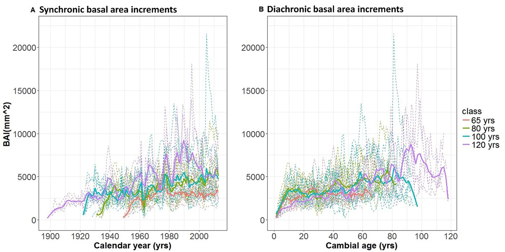
The basal area increments of trees belonging to the different age classes are presented in Fig. 2a and Fig. 2b, plotted against calendar year and cambial age, respectively. Taking a synchronic perspective, BAI shows a distinct increase over the last century, with values for some trees reaching above 10.000 mm2 yr-1. In the 1950-2010 period covered by all four age classes, younger trees seem to present slower growth rates than older individuals. Such an age-related pattern is confirmed by the diachronic analysis of Fig. 2b, which suggests a continuous increase in basal area increments until an age of 90 years; the sharp drop at the far end of the 100- and 120-year age classes is an artifact, due to the declining number of trees reaching the oldest age in each class. The diachronic perspective also reveals, however, that global change also contributes to the observed time dynamics, as young trees are currently growing less than similarly aged trees 40 to 60 years ago.
Fig. 2 - Dynamics of basal area increments (BAI) in different age-classes. BAI time series for single tree chronologies (dashed lines) and after grouping by age-class and fitting with a cubic spline (continuous lines) are presented (A) in a synchronic (i.e., against calendar year) and (B) in a diachronic perspective (i.e., against cambial age).
Model output
In order to assess possible changes of growth rates over time, independent of the co-occurring effects of ontogenetic factors, tree basal area increments (BAI) were modeled as (eqn. 3):
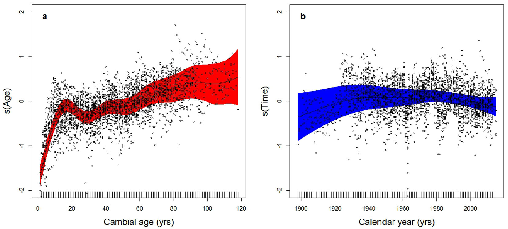
where s(Age) is the cambial age effect and s(Time) represents all of the environmental effects cumulated into a single global change variable, varying over time. The age-related effect (Fig. 3a) displays the expected shape, with a steep increase at early age in the first part of the curve, followed by a less pronounced growth, and an apparent flattening at an age of 90. After the subtraction of the age-related signal, the trend in the BAI component associated with global change (Fig. 3b) shows an initial increase, two culminations around the ’30s and the ’80s of the last century, a lower growth in between and a subsequent decrease until the first decade of this century, which is significant at the 95% level.
Fig. 3 - GAMM analysis of the independent effects of age and time on basal area increments (BAI - see eqn. 3). (a) Trend of log(BAI) as a function of age alone after correcting for time-related effects. On the x-axis is cambial age (years), on y-axis is s(Age), the component of log(BAI) explained by age, dimensionless and centered around 0. (b) Trend of log(BAI) as a function of time alone, after correcting for age-related effects. On x-axis is calendar year, on y-axis is s(Time), the component of log(BAI) explained by time per se, dimensionless and centered around 0. Points represent partial residuals from the fitted function and the shaded areas indicate the 95% prediction interval of fitted adaptive splines. The GAMM model of eqn. 3 was applied to log-transformed BAI data, so as to correct for heteroscedasticity.
As a second step, in order to partition to individual drivers the effect so far attributed to global change, seasonal climatic (temperature and SPEI) and geochemical variables (atmospheric [CO2] and N deposition) were added to the model instead of time per se.
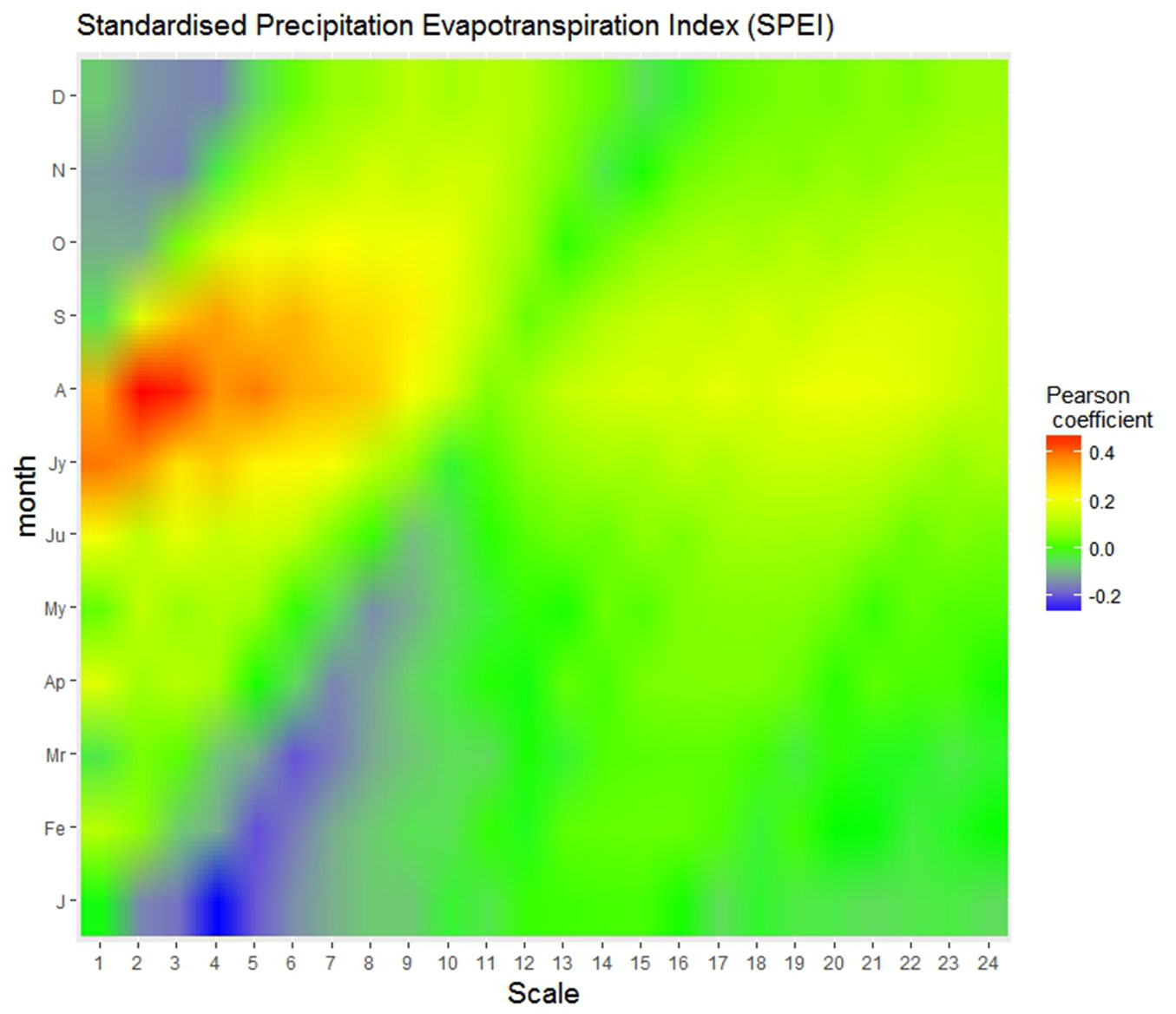
In a preliminary analysis, the SPEI index most correlated with RWI was found to be centered on August with a two-months timescale (hence referred to as SPEIJA), with a Pearson’s correlation coefficient of 0.46 (Fig. 4); this suggests a short-time response to drought, which is typical of a highly productive coniferous forest in such a mesic environment. A two-months timescale was therefore assumed for SPEI in all subsequent analyses.
Fig. 4 - Heatmap of SPEI correlation with ring-width index (RWI) series. Correlation (Pearson’s coefficient) between de-trended tree-ring index (RWI) and the Standardized Precipitation Evapotranspiration Index (SPEI) computed for different months (on the y-axis) and temporal scales ranging from 1- to 24 months.
Tab. 3 - Differences in the Bayesan information criterion (ΔBIC) of alternative log(BAI) GAMM models. The selected model with the lowest BIC is marked with an asterisk (*). ΔBIC was calculated as the difference between the BIC of each model and that of the selected model. (Age): cambial age; (CO2): atmospheric [CO2]; (Ndep): atmospheric N deposition; (SPEI): Standardized Precipitation Evapotranspiration Index (SPEI) in July and August of the current year; (SPEI t-1): SPEI in August and September of the previous year; (T): mean temperature of January-March period of the current year. All models are subsets of the full model (m0).
| Model fixed effects | Model | BIC | ΔBIC |
|---|---|---|---|
| Age +CO2 +Ndep +SPEI +SPEIt-1 +T | m0 | -40.6947 | 20.6109 |
| CO2 +Ndep +SPEI +SPEIt-1 +T | m1 | 164.3962 | 225.7018 |
| Age +Ndep +SPEI +SPEIt-1 +T | m2 | -46.7642 | 14.5414 |
| Age +CO2 +SPEI +SPEIt-1 +T | m3 | -24.8838 | 36.4219 |
| Age +CO2 +Ndep +SPEIt-1 +T | m4 | 49.7032 | 111.0088 |
| Age +CO2 +Ndep +SPEI +T | m5 | -17.9830 | 43.3226 |
| Age +CO2 +Ndep +SPEI +SPEIt-1 | m6 | 144.5604 | 205.8660 |
| Ndep +SPEI +SPEIt-1 +T | m7 | 202.7464 | 264.0520 |
| Age +SPEI +SPEIt-1 +T | m8 * | -61.3056 | - |
| Age +Ndep +SPEIt-1 +T | m9 | 43.6166 | 104.9222 |
| Age +Ndep +SPEI +T | m10 | -40.8651 | 20.4405 |
| Age +Ndep +SPEI +SPEIt-1 | m11 | 117.4654 | 178.7710 |
| SPEI +SPEIt-1 +T | m12 | 339.8094 | 401.1150 |
| Age +SPEIt-1 +T | m13 | 32.7605 | 94.0661 |
After a procedure of backward stepwise variable selection (Tab. 3), the resulting model was specified as follow (eqn. 4):
where Age is the age-size effect associated with variations in cambial age, SPEIJAt and SPEISAt-1 represent the SPEI (indicative of water availability and drought stress) of the current summer (July and August) and of the end of the previous growing season (August and September), respectively, and TJFMt is the mean temperature of January, February and March of the current year. In addition to age, the latter appears to be the most important environmental factor explaining the long-term growth trend in the Douglas fir chronosequence (F-test = 35.25), followed by the SPEI index for the ongoing season (F-test = 20.607) and the SPEI index representing water availability at the end of previous growing season (F-test = 11.255). All variables exhibit a significant p-value at 0.001 level (Tab. 4), with a global adjusted R2 for the whole model of 0.564.
Tab. 4 - Generalized additive mixed model (GAMM) results for the relationship between the logarithm of basal area increments (BAI) and climatic and biological factors in Pseudotsuga menziesii, as presented in eqn. 4. (edf): effective degrees of freedom; (F): F-test for variance explained; (P): p-values; (R2-adj): adjusted regression coefficient of the model.
| Factor | edf | F | P | R 2 -adj |
|---|---|---|---|---|
| Age | 8.479 | 57.273 | < 2e-16 | - |
| SPEIJAt | 5.53 | 20.607 | < 2e-16 | - |
| SPEIASt-1 | 7.473 | 11.255 | 2.58e-16 | - |
| TJFMt | 5.859 | 35.25 | < 2e-16 | - |
| s(series) | 25.682 | 3.165 | 9.02e-15 | - |
| Whole model | - | - | - | 0.564 |
Discussion
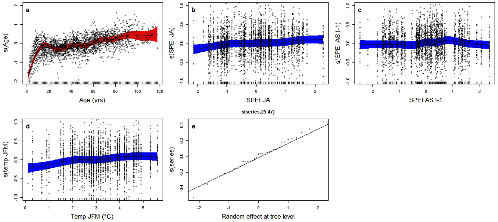
The primary purpose of this study was to assess if any changes in growth rates have occurred over the last century in Douglas fir stands growing in the northern Apennines, after correcting for age-related patterns. The analysis of age-adjusted long-term trends indeed demonstrates a significant decrease in the productivity of this species from its peak value in the 1980s. These findings appear to be consistent with several other studies that looked at forest growth changes in central Apennines ([34]), in the Mediterranean region by and large ([24]) and in other European areas ([42]). The increase in summer drought resulting from increasing temperatures in recent years was generally found to have had a negative effect on growth, in association with co-varying factors, such as stand dynamics, competition and pests. These could exacerbate the role of the imbalance in water availability and overcome the potentially positive effects of the increase in the length of the growing season induced by higher temperatures and of the rise in atmospheric [CO2], as well as of atmospheric N deposition. The general trend recorded in this study can be partially explained by examining the shape of the relationship between significant environmental factors and BAI. The effect of age displays, after an initial abrupt increase, a successive phase of rather constant rise and an apparent stabilization of growth at advanced age, largely consistent with what already observed in the preliminary analysis. The quasi-linear positive relationship between growth and mean winter-spring temperature (Fig. 5d) probably reflects the beneficial effect that high temperatures have at mountain sites, by reducing frost damage, snow accumulation and maintaining significant carbon assimilation during the dormant season, even at minimum photosynthetic rates ([14]), as well as inducing a longer vegetative season. Summer water availability (Fig. 5b), which is related to both precipitation and transpiration demand, is the third most important variable affecting the behavior of this species in the long-term, conditioning its growth performance ([5]) and distribution ([36]). Air dryness, which is also known to affect Douglas fir, was not included as a potential driver in the present study due to a lack of suitable information. Water availability at the end of the previous growing season (August-September - Fig. 5c) was also expected to have a positive effect on growth, since early-wood width is related to the amount of carbon storage reserves built-up in the preceding year, which are subject to remobilisation in the first phase of vegetative growth ([22]). The shape of the relationship in Fig. 5c, however, suggests no negative effects of late-summer water deficit but on the contrary a slightly significant detrimental effect of water surplus. This behavior could be associated with the reduction of solar radiance, due to intense precipitation which can lead to an earlier end of the vegetative period.
Fig. 5 - GAMM analysis of the independent effects of individual drivers on basal area increments (BAI - see eqn. 4). Generalized additive model (GAMM) results show the component of log(BAI) (dimensionless and centered around 0) explained by individual environmental and biological factors remaining after the backward model selection procedure: (a) cambial age; Standardized Precipitation Evapotranspiration Index computed over (b) July and August of the current year (SPEIJA) and (c) August and September of the previous year (SPEIASt-1); and (d) mean temperature over January, February and March (TempJFM). Points represent partial residuals from the fitted function and the shaded areas indicate the 95% prediction interval. The GAMM model was applied to log-transformed BAI data, so as to correct for heteroscedasticity.
The lack of evidence of a fertilization effect of CO2 is in agreement with previous studies ([23]) and could lead to different conclusions, depending on the processes involved. From a biological perspective, for example, both long-term photosynthetic acclimation ([29]) and a shift in allocation of assimilated C to faster-turnover pools such as fine roots or canopy foliage ([21]) are possible explanations; taking a more biogeochemical perspective, this lack of response could also be attributed to the emergence of nutrient limitations, as nutrient availability cannot keep up with increasing C assimilation ([31]).
It is important to recognize, however, that our results could be affected by a number of potential artifacts. First of all, the lack of a CO2 fertilization effect could be due to the addition of the AR(1) structure for autocorrelation, since atmospheric [CO2] is very similar from year to year and its incremental effects could be falsely attributed to previous year’s growth.
Our assumption of no competition effects could also have biased the results. The growth of shade intolerant trees is significantly affected by stand density, especially in even-aged stands. Although the sampled trees have long maintained their dominant status (see Supplementary material) and should be therefore considered exempt from severe competition and growth suppression, we cannot exclude the presence of a positive influence of thinning (i.e., release effect - [16]), which is recognized to enhance tree growth also at advanced age ([26]).
The impact of drought events could also have been insufficiently represented by the rather crude approach applied in the study. Finally, it should be mentioned that, when non-stationary forcing factors (i.e., atmospheric [CO2] and N deposition) co-vary, it is difficult to disentangle their individual effects on long-term tree growth, and this complication increases with the complexity of the model ([10]).
Conclusions
The combination of the chronosequence approach with Generalized Additive Mixed Models appears to have real potential to disentangle the superimposed non-linear biological and environmental effects affecting tree growth. By avoiding any de-trending with an a priori model structure, the technique results in long-term trend preservation, which is fundamental to better understand past environmental effects and to predict the future behavior of forests in a changing world.
Given the importance of Douglas fir as a timber species, the ongoing decrease in growth performance illustrated by this study for the northern Apennines could have relevant implications from a management perspective. For this reason, understanding which factors have been determining such a trend is particularly important. Our model, despite the rather low amount of variance explained and the simplicity of the model structure, considering only a limited number of variables, allows us to draw some conclusions. The impact of summer water availability, which is projected to decrease in the Mediterranean region ([20]), could be responsible to a considerable extent for the observed decrease in growth rates in recent decades, due to the increase in magnitude and frequency of drought events. The positive effect ascribable to the extension of the growing season, as a result of increasing winter-spring temperatures, which should have promoted stem growth in the past, may no longer be able to counterbalance this summer drought stress effect. Especially in the absence of a positive effect of fertilization by rising atmospheric [CO2] and N deposition, the observed trend can be expected to be exacerbated in the future.
Acknowledgments
We thank NOAA (ITRDB and ESRL) and the Regional Hydrological Service of the Tuscany Region (SIR), for providing the environmental data used in this study; also the Ufficio Territoriale Carabinieri per la Biodiversità di Vallombrosa which kindly provided sampling permission.
This work was carried out within the framework of the Convention between the Department of Agricultural and Food Sciences of the University of Bologna and the CREA Research Centre for Forestry and Wood.
References
Gscholar
Gscholar
CrossRef | Gscholar
Gscholar
Gscholar
CrossRef | Gscholar
CrossRef | Gscholar
Gscholar
Gscholar
Gscholar
Authors’ Info
Authors’ Affiliation
Federico Magnani 0000-0003-4479-0916
Dipartimento di Scienze e Tecnologie Agro-Alimentari, Alma Mater Studiorum - Università di Bologna, via Fanin 44, I-40127 Bologna (Italy)
CREA Research Centre for Forestry and Wood, v.le Santa Margherita 80, I-52100 Arezzo (Italy)
Corresponding author
Paper Info
Citation
Ravaioli D, Ferretti F, Magnani F (2019). Disentangling the effects of age and global change on Douglas fir growth. iForest 12: 246-253. - doi: 10.3832/ifor2620-012
Academic Editor
Marco Borghetti
Paper history
Received: Sep 01, 2017
Accepted: Mar 11, 2019
First online: May 03, 2019
Publication Date: Jun 30, 2019
Publication Time: 1.77 months
Copyright Information
© SISEF - The Italian Society of Silviculture and Forest Ecology 2019
Open Access
This article is distributed under the terms of the Creative Commons Attribution-Non Commercial 4.0 International (https://creativecommons.org/licenses/by-nc/4.0/), which permits unrestricted use, distribution, and reproduction in any medium, provided you give appropriate credit to the original author(s) and the source, provide a link to the Creative Commons license, and indicate if changes were made.

Web Metrics
Breakdown by View Type
Article Usage
Total Article Views: 46054
(from publication date up to now)
Breakdown by View Type
HTML Page Views: 38652
Abstract Page Views: 3537
PDF Downloads: 2869
Citation/Reference Downloads: 8
XML Downloads: 988
Web Metrics
Days since publication: 2635
Overall contacts: 46054
Avg. contacts per week: 122.34
Article Citations
Article citations are based on data periodically collected from the Clarivate Web of Science web site
(last update: Mar 2025)
Total number of cites (since 2019): 6
Average cites per year: 0.86
Publication Metrics
by Dimensions ©
Articles citing this article
List of the papers citing this article based on CrossRef Cited-by.
Related Contents
iForest Similar Articles
Research Articles
Role of photosynthesis and stomatal conductance on the long-term rising of intrinsic water use efficiency in dominant trees in three old-growth forests in Bosnia-Herzegovina and Montenegro
vol. 14, pp. 53-60 (online: 28 January 2021)
Technical Advances
Improved estimates of per-plot basal area from angle count inventories
vol. 7, pp. 178-185 (online: 17 February 2014)
Research Articles
Growth dynamics and productivity of pure and mixed Castanea sativa Mill. and Pseudotsuga menziesii (Mirb.) Franco plantations in northern Portugal
vol. 7, pp. 92-102 (online: 18 December 2013)
Progress Reports
Basic concepts and research activities at Italian forest sites of the Long Term Ecological Research network
vol. 4, pp. 233-241 (online: 04 November 2011)
Research Articles
Climate impacts on tree growth in a Neotropical high mountain forest of the Peruvian Andes
vol. 13, pp. 194-201 (online: 19 May 2020)
Research Articles
Scots pine’s capacity to adapt to climate change in hemi-boreal forests in relation to dominating tree increment and site condition
vol. 14, pp. 473-482 (online: 18 October 2021)
Research Articles
Spatio-temporal modelling of forest monitoring data: modelling German tree defoliation data collected between 1989 and 2015 for trend estimation and survey grid examination using GAMMs
vol. 12, pp. 338-348 (online: 05 July 2019)
Editorials
COST Action FP0903: “Research, monitoring and modelling in the study of climate change and air pollution impacts on forest ecosystems”
vol. 4, pp. 160-161 (online: 11 August 2011)
Research Articles
High resolution biomass mapping in tropical forests with LiDAR-derived Digital Models: Poás Volcano National Park (Costa Rica)
vol. 10, pp. 259-266 (online: 23 February 2017)
Research Articles
Local ecological niche modelling to provide suitability maps for 27 forest tree species in edge conditions
vol. 13, pp. 230-237 (online: 19 June 2020)
iForest Database Search
Search By Author
Search By Keyword
Google Scholar Search
Citing Articles
Search By Author
Search By Keywords
PubMed Search
Search By Author
Search By Keyword


