Regional-scale stand density management diagrams for Pyrenean oak (Quercus pyrenaica Willd.) stands in north-west Spain
iForest - Biogeosciences and Forestry, Volume 6, Issue 3, Pages 113-122 (2013)
doi: https://doi.org/10.3832/ifor0880-006
Published: Mar 05, 2013 - Copyright © 2013 SISEF
Research Articles
Abstract
Stand Density Management Diagrams are useful tools for designing and evaluating alternative density management regimes without the need of implementing any silvicultural action, and allowing the future stand conditions to be predicted prior to implementing management schedules. In this study, stand density management diagrams were developed for Pyrenean oak (Quercus pyrenaica Willd.) stands in north-west Spain by including data on stand volume, stand aboveground biomass, stand stem biomass and carbon pools. Data were obtained from Third National Forest Inventory plots (n=1860). The large geographical area analyzed in this study was classified by provenance regions, which were compared in terms of biomass production in order to define areas with similar characteristics for use as management units. The comparisons identified 6 independent groups. Different stand-level models and the associated diagrams for the aforementioned stand variables were therefore developed for each group.
Keywords
SDMDs, Pyrenean Oak, Rebollo Oak, Biomass, Forest Management
Introduction
From the early days of forestry, one of the main aims of managers and researchers has been to estimate forest production and, more problematically, to predict productivity well before harvesting ([68]). This can be achieved in two different ways: by considering environmental factors and by measuring stand parameters as indicators of the site and/or forest productivity ([11]). The second option has been found to be clearer, simpler and more reliable ([15]).
Several studies published during the 1950s and 1960s showed that stand development and forest productivity, including self-thinning and other competitive effects at tree and stand levels, are mainly influenced by stand density ([42], [43], [60], [70]). According to Jack & Long ([39]), forests can be managed by controlling only stand density. Conceptually, stand density management is the process of controlling resource competition through density regulation to meet specified management objectives ([52]). However, at the operational level, density regulation consists in controlling the level of growing stock through initial spacing and/or subsequent thinning ([12]).
Conversion of these specific management objectives into appropriate upper and lower levels of growing stock at stand level (expressed by the relative spacing index) is the most difficult step in designing a density management regime ([24], [22]). According to Dean & Baldwin ([26]), the upper level is chosen to yield acceptable stand growth and individual tree vigor, while the lower level is chosen to maintain acceptable site occupancy. These must therefore be constrained within stand densities corresponding to the threshold of self-thinning and canopy closure ([26]). According to Jack & Long ([39]), the use of experimental thinning plots is the best option for determining the theoretical limits mentioned above. However, there are two serious disadvantages associated with the use of such plots ([25]): they are long-lasting and the results cannot be extrapolated accurately to forest stands with different site quality or management objectives.
One useful alternative approach for forest management decision-making is to use Stand Density Management Diagrams (SDMDs), which provide resource managers with an objective method of determining density control schedules ([52]) and integrate relationships between density, stand structure, canopy dynamics and production efficiency, linking quantitative silviculture to population ecology, production ecology and biometrics ([39]). The first diagrams were constructed by Ando ([10]), who presented the competition and yield equations (based on stand density) and the self-thinning rule in a two-dimensional graphical format, which allowed thinning regimes to be derived in relation to management objectives. Several additions and modifications to the original modelling approach were proposed later on ([64], [4], [31], [32], [48]), including the replacement of the original yield-density equations with empirical-based volume-density functions ([53]) and the application of different relative density indexes ([52]).
SDMDs are therefore graphical tools used in the design of silvicultural regimes in even-aged forests to illustrate the relationships between yield, density and mortality throughout all stages of stand development ([54]). They also enable the simulation of several management regimes and the development of thinning schedules for a wide range of site qualities and management objectives ([21]), by using indices that relate the average tree size (e.g. volume, height or diameter) to density (e.g. number of trees per hectare - [12]); this ensures that tree size is independent from site quality and stand age ([48]). SDMDs can also be used to control shrub development during early stages of stand development ([62]), reduce stand susceptibility to pests ([45]) and optimize wildlife habitat ([63]). However, their use is limited to a geographic range similar to that used for diagram calibration ([31]).
Quercus pyrenaica Willd. is a deciduous Mediterranean species, whose natural range is in south-western Europe ([56]). More specifically, its distribution area includes Portugal (62 000 ha), Spain (660 000 ha), western France (34 500 ha) and northern Morocco (5 000 ha - [19]). Spain and Portugal represent about 95% of the natural distribution area, so that the species can almost be considered as endemic to the Iberian Peninsula ([46]).
From a biogeographical point of view, Q. pyrenaica occupies an intermediate position between the central European Atlantic deciduous forests and Mediterranean xerophytic formations in the south of the Iberian Peninsula ([19]), and its water and soil requirements are also intermediate between those of pure Atlantic (e.g., Quercus robur L.) and pure Mediterranean oaks (e.g., Quercus ilex L. - [23]).
Owing to the wide distribution of Q. pyrenaica, there is great variability among stands of this species in Spain in terms of silvicultural and ecological conditions ([2]). Furthermore, traditional treatments, pasture and forest fires have also affected Q. pyrenaica stands, further contributing to their variability ([5]). As a result of these driving factors, Pyrenean oak stands are mainly found in the form of coppice- managed stands or young forests, ranging from diminished stands with low densities to open woodlands with large diameter trees ([1], [56]). The current extension of the species’ range is lower than its potential distribution ([58]), probably because of the common replacement of Pyrenean oak stands by more productive pine plantations ([50]). Nevertheless, species’ covering in Spain doubled between the Second and the Third National Forest Inventories (period 1996-2006 - [27]), and some authors ([35]) hypothesized that climate change might favor the expansion of its natural range.
According to Adame et al. ([1]), management of oak forests is one of the greatest problems that forestry research is facing in Spain. It can be assumed that during at least the last 50 years, the average rotation length for Mediterranean coppices in Spain has varied between 20 and 30 years as a consequence of variations in the economy and the sociology of rural areas ([1]). The increased migration of rural populations to urban areas is leading to abandonment of traditional uses of oak (for firewood and charcoal), so that indirect uses of these forests (i.e., silvopastoral uses, recreation, protection against erosion, regulation of water regime, etc.) and environmental functions (particularly their role of carbon sinks) have become more and more important ([20]).
This has promoted interest in the structure, function and dynamics of these forest ecosystems, hitherto poorly known, despite being the fifth most important forest species in the Iberian Peninsula ([58]). As a result of this interest, a wide range of studies have been published in the last few decades. These studies have included the following aspects (amongst others): development of site index curves, in León ([66]), La Rioja ([15]), Castilla y León ([1]) and Galicia ([29]); fitting height-diameter models ([2]); modeling mortality ([3]); stand yield in terms of biomass ([6], [19]); and estimation of carbon stocks in Pyrenean oak stands, both in soils ([30]) and in wood ([20]). However, only one stand-level model has been developed to date and this refers to the province of Leon ([16]).
The aim of the present study was to develop practical SDMDs to provide a tool to help forest managers in the decision-making process (specifically those associated with the management of pure Pyrenean oak stands in north-west Spain) and to assess the aboveground wood volume. Forest managers can use these diagrams to plan different thinning regimes on the basis of current tree spacing and thus anticipate when the Pyrenean oak stand will be overcrowded. Foresters are usually unwilling to cut sufficient numbers of trees during thinning to allow the remaining trees to grow vigorously, and SDMDs will provide them with an objective means for determining the appropriate stand spacing.
Material and Methods
Data
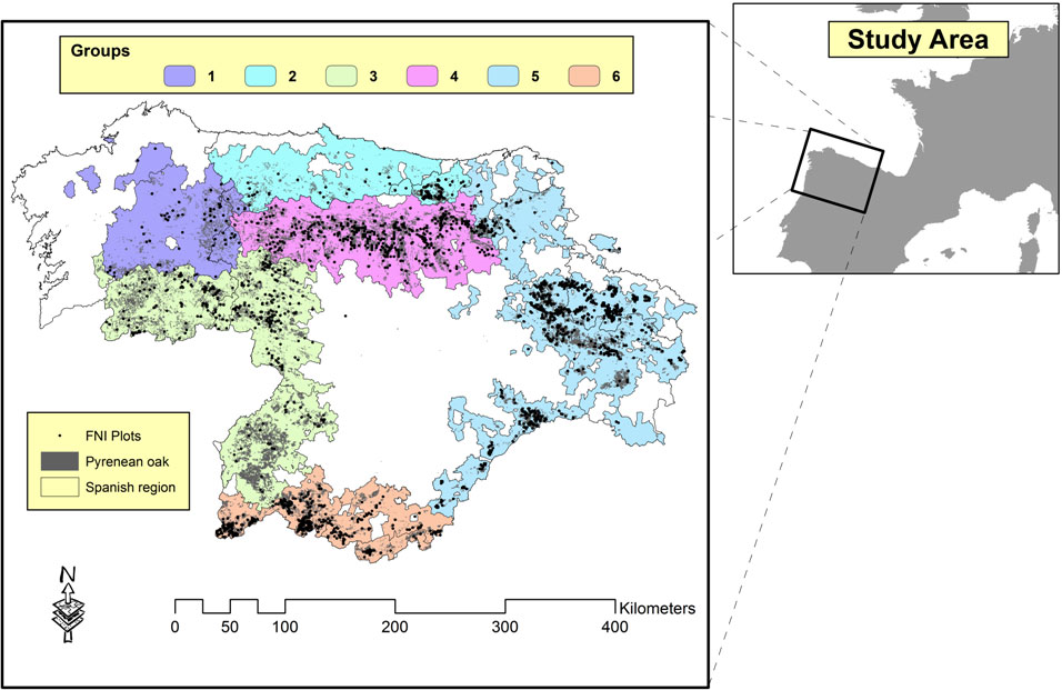
Data used to develop the SDMDs for Pyrenean oak stands in NW Spain were obtained from the Third Spanish National Forest Inventory (NFI) plots ([27]) throughout the regions of Galicia, Asturias, Cantabria, La Rioja and Castilla y León. These consist of a systematic sample of permanent plots located on the nodes of a 1 km UTM square grid, comprising four sub-plots of radius of 5, 10, 15 and 25 m, with a minimum diameter at breast height threshold of 75, 125, 225 and 425 mm, respectively, and with a re-measurement interval of 10 years. Among all the NFI plots, those where Pyrenean oak was the dominant species (basal area proportion > 90%), with a stand density higher than 100 trees ha-1, were selected (n = 1860). According to Bravo et al. ([18]), the limit between open woodlands (in Spanish: dehesa) and Pyrenean oak forests (both high and coppice forests) is 100 trees ha-1.
Although the Pyrenean oak is widely distributed throughout the Iberian Peninsula, it is mainly found in the northwestern mountainous ranges ([23]). Indeed, the aforementioned regions account for more than 85% of the total species’ covering in Spain ([27]). Within this large area many different soil and climatic conditions can be found ([57]), including different bedrock substrates (granite, gneiss, quartzite, slate, etc.) and soils (Cambisols and rankers), although the most important is the common siliceous substrate ([40]). Furthermore, the study area includes both Atlantic and Mediterranean regions that differ significantly in terms of rainfall and temperature ([23], [57]). The above variability is reflected in the presence of different plant species making up different geobotanical associations throughout the study area. The following species appear in Atlantic environments (e.g., Galicia and Asturias): accessory shrub species, such as Cytisus cantabricus, C. multiflorus, C. striatus, Erica arborea, E. cinerea, Calluna vulgaris, Genista florida sbsp. polygaliphylla, and herbaceous species, such as Melampyrum pratense, Linaria triornitophora, Holcus mollis, Deschampia flexuosa, Poa nemoralis ([28], [23]), which are replaced by others, such as Genista falcata, Cytisus purgans, Adenocarpus hispanicus, Satureja vulgaris, Arenaria montana, Geum sylvaticum, Veronica officinalis, Viola riviniana, V. odorata, Luzula forsteri, in Mediterranean environments ([50], [23]). Likewise, areas with intermediate conditions between Atlantic and Mediterranean environments have their own accessory species ([50]). For more details about geobotanical associations and accessory species in Spanish Q. pyrenaica stands, see Mesón García ([50]), Jiménez-Sancho et al. ([40]), Costa et al. ([23]) and Ruiz de la Torre ([56]).
Several studies have delimited zones of similar characteristics within the wide geographical area considered in the present study, which could be used as management units. These zones vary from bioclimatic ecoregions ([33]) to genetic provenance regions ([40]). The difference between both categories is straightforward: an ecoregion is delimited by physiographic and climatic conditions ([33]), while a provenance region is species-specific and reflects the region where species’ populations share a similar phenotypic and/or genetic make-up, i.e., it may include a set of intermixable populations suffering similar selective pressures ([40]). Therefore, at species level, geographic differentiation by provenance regions would be more reliable than differentiation by ecoregions.
Based of the above considerations, each plot was assigned to its respective provenance region by spatial data analysis, by use of a Geographical Information System ([34]). Fifteen provenance regions were identified within the database: (1) Galicia septentrional; (2) Galicia meridional; (3) Aliste-Maragatería; (4) Cordillera Cantábrica meridional; (5) Cordillera Cantábrica oriental; (6) Sistema Ibérico septentrional; (7) Salamanca-Sayago; (8) Gata y Peña de Francia; (9) Gredos y Sierra de Ávila; (10) Valles del Tiétar y Jerte; (11) Norte de la Sierra de Guadarrama; (13) Sistema Ibérico meridional; (A) Rías Altas, (C) Asturias; and (D) La Liébana ([40]).
Moreover, the following stand variables were calculated for each plot: number of trees per hectare (N), quadratic mean diameter (dg), dominant height (H0 - defined as the mean height of the 100 thickest trees per hectare), total stand volume (Vcc), stand stem biomass (Wf) and stand aboveground biomass (Wt). The total stand volume was calculated by summing the individual volumes and considering the expansion factors for each sub-plot, according to Bravo et al. ([17]). Stand stem and stand aboveground biomass were calculated from the individual equations developed for these types of forests by Carvalho ([19] - eqn. 1, R2adj = 0.991, E = 0.117 Kg) and Montero et al. ([51] - eqn. 2, R2adj = 0.978, E = 0.247 Kg), respectively, by a scaling-up approach. This method allows the prediction of stand biomass as the sum of the values predicted for individual trees (eqn. 1-2).
where Wf is the stand stem biomass (Mg ha-1), Wt the stand aboveground biomass (Mg ha-1), d is diameter at breast height (cm), h is total tree height (m), R2adj is the adjusted coefficient of determination, and E is the mean bias.
Construction of the SDMDs
SDMDs consist of a system of four equations and the relative spacing index (RS) as basic components. The RS is used to characterize the growing stock level and is calculated as the ratio, expressed as a percentage, between the average distance among trees and the dominant height. This index, which was first proposed for plantations by Hart in 1928, was later referred to as the spacing index by Becking in 1954, and as relative spacing by Clutter et al. ([22]) and Gadow & Hui ([36]). RS is useful in stand density management because it is independent of site quality and stand age, except in very young stands, and because from a biological point of view, dominant height is one of the best criteria for establishing thinning intervals ([12]). The association between dominant height growth and forest production adds further utility to these diagrams for forest management purposes ([13]). As Q. pyrenaica stands are natural forests that are influenced by management (e.g., as a source of firewood), we assumed a triangular spacing between trees, so that RS can be expressed as follows (eqn. 3):
where RS is the relative spacing index (%), N is the number of stems per hectare, and H0 is the dominant height (m).
The first step in the construction of the SDMD is to fit the non-linear system of the following four equations (eqn. 4-eqn. 7):
where N is the number of stems per hectare, dg is the quadratic mean diameter (cm), H0 is the dominant height (m), V the stand volume (m3 ha-1), Wf the stand stem biomass (Mg ha-1), Wt the stand aboveground biomass (Mg ha-1) and βi (i = 0, 1, …, 14) are the regression coefficients to be estimated.
Equations 4-7 together define a structurally simultaneous system of equations, where N and H0 are exogenous variables, V, Wf and Wt are endogenous variables and dg is an endogenous instrumental variable. As there is correlation between the error components of the variables on the left-hand side and the right-hand side, the full information likelihood technique was applied to fit all the equations simultaneously by use of the MPEFM procedure of SAS/ETS® ([59]).
Comparisons of different regions
Forest site productivity can be defined as the potential of a particular forest stand to produce aboveground wood volume, where the production unit refers to the site and the tree stand together ([61]). Estimation of stem volume is important for mapping standing stock and for forest inventory purposes because it provides initial prediction of the amount of timber that could be commercially harvested ([69]), so that the maximum mean annual volume increment is usually considered a suitable measure of site quality. However, the volume attained by a stand at any given age can be affected by factors other than site quality, and unless these factors are controlled or adjustments are made to reflect their effects, differences in volumetric production among forest stands will bear little relationship to true differences in site quality. The principal confounding factors are stand density, species composition, genetics and cultural practices ([22]).
Measurement of biomass is a parameter suitable for assessing the structure, functions and dynamics of forest ecosystems ([19], [51]) and for estimating carbon sequestration in a forest region over time ([37]) because changes in biomass are linked with important outcomes in ecosystem functional characteristics and climate change. In fact, accurate assessment of biomass at local to regional and global scales becomes important for reducing the uncertainty of environmental processes and sustainability ([65]). Therefore, biomass is considered better than volume for forest stands comparison purposes.
Moreover, estimation of the forest carbon (C) pool also provides an important indicator of sustainable forest management (well-managed forestland) in forest certification assessment (for instance in the Pan-European Criteria and Indicators for Sustainable Forest Management - [49]). The carbon content of trees is usually calculated from wood volume equations (m3) that include basic wood density (Mg m-3) and a conversion factor for the C concentration in dry biomass (% C - [37]). In this study, the carbon pool was calculated directly from stand aboveground biomass (Mg ha-1) and a specific conversion factor was applied for Pyrenean oak (0.475, according to [51]).
The Lakkis-Jones test (eqn. 8 - [41]) and the non-linear extra sum of squares method (eqn. 9 - [14]) have been applied to the analysis of differences among geographic regions (e.g. [8], [13], [2]). In the present study, both methods were used for the simultaneous detection of homogeneity among the regression coefficients of the stand aboveground biomass equation (eqn. 7) for the 15 previously defined provenance regions. The aforementioned comparative methods require fitting of reduced and full models. While the reduced model has the same set of parameters for all regions, the full model corresponds to different sets of parameters for each group and is obtained by expanding each parameter through an associated parameter and a dummy variable to differentiate the regions. The expressions are as follows (eqn. 8-9):
where L is the Lakkis-Jones value, FChow is the non-linear sum of squares method value, SSEF refers to the error sum of squares of the full model, SSER is the error sum of squares of the reduced model, n is the number of data in the reduced model, and dfR and dfF are the degrees of freedom associated with the reduced and full model, respectively.
Based on the results of previous comparisons, we proceeded to refit the non-linear system of equations (eqn. 4-eqn. 7) simultaneously for each group derived from the above analysis.
SDMDs graphical representation
The final step in the construction of the SDMDs consists of representing the isolines for the growing stock (expressed by the RS) and for the stand variables included in the stand-level model (dg, V, Wf and Wt).
Several different methods have been used to construct SDMDs ([39]). In the system proposed here, dominant height was represented on the x-axis and the number of trees per hectare in logarithmic scale on the y-axis, following the method proposed by Barrio-Anta & Álvarez-González ([12]). The isolines were obtained by solving for N in eqn. 3-7 (see [13], for more details). The quadratic mean diameter isolines were represented in the diagrams, using constant values for dg and solving eqn. 4 for N. However, the isolines for eqn. 5-eqn. 7 were represented in the diagrams by solving dg in each equation with eqn. 4, assuming constant values for each variable and solving for N.
Results and discussion
Comparison among provenance regions
The significant values for the Lakkis-Jones and the non-linear extra sum of squares tests are shown in Tab. 1, along with the regression statistics of the reduced and full models of eqn. 7. The results revealed the formation of 6 independent groups, which are illustrated in Fig. 1. The stand variable summary statistics (mean, maximum, minimum and standard deviation) are shown in Tab. 2.
Tab. 1 - Goodness-of-fit statistics and results of the non linear extra sum of squares (F-value) and the Lakkis and Jones (Lakkis value) tests used to examine regional differences between the reduced and full models. Only the significant differences are shown. (PR): Provenance Regions for Pyrenean oak in Spain ([40]); (SSE): sum of squared errors; (df): degrees of freedom; (MSE): mean squared error; (R2): coefficient of determination for non-linear regression; (n): sample size. (*): p < 0.05.
| Comparison | Reduced model | Full model | R2 | n | F-value | Lakkis value |
||||
|---|---|---|---|---|---|---|---|---|---|---|
| SSE | df | MSE | SSE | df | MSE | |||||
| PR_1 vs. PR_A | 1611.9 | 63 | 25.58 | 1609.4 | 60 | 26.82 | 0.9945 | 66 | 0.0314 * | 0.1036 * |
| PR_C vs. PR_D | 28579.6 | 84 | 340.2 | 26134 | 81 | 322.6 | 0.9603 | 87 | 2.5266 * | 7.7826 * |
| PR_2 vs. PR_3 | 6676.6 | 239 | 27.93 | 6638.4 | 236 | 28.13 | 0.9916 | 242 | 0.4494 * | 1.3785 * |
| PR_2 vs. PR_7 | 3643.6 | 136 | 26.79 | 3460.2 | 133 | 26.01 | 0.9941 | 139 | 2.3489 * | 7.1763 * |
| PR_3 vs. PR_7 | 3656.8 | 168 | 21.77 | 3525.3 | 165 | 21.36 | 0.9835 | 171 | 2.0522 * | 6.2642 * |
| PR_5 vs. PR_6 | 103828 | 575 | 180.6 | 102804 | 572 | 179.7 | 0.9679 | 578 | 1.8693 * | 5.7293 * |
| PR_5 vs. PR_11 | 3404.4 | 191 | 17.82 | 3380 | 188 | 17.98 | 0.9895 | 194 | 0.4513 * | 1.3923 * |
| PR_5 vs. PR_13 | 1827.3 | 64 | 28.55 | 11769.8 | 61 | 192.9 | 0.9860 | 67 | 1.0267 * | 4.9898 * |
| PR_6 vs. PR_11 | 103977 | 639 | 162.7 | 102536 | 636 | 161.2 | 0.9693 | 642 | 2.2275 * | 8.9597 * |
| PR_6 vs. PR_13 | 101065 | 512 | 197.4 | 100980 | 509 | 198.38 | 0.9667 | 515 | 0.1065 * | 0.4324 * |
| PR_11 vs. PR_13 | 1557.4 | 128 | 12.16 | 1556 | 125 | 12.45 | 0.9903 | 131 | 0.0277 * | 0.1179 * |
| PR_8 vs. PR_9 | 5787.2 | 316 | 18.31 | 5644 | 313 | 18.03 | 0.9919 | 319 | 2.6479 * | 7.9950 * |
| PR_8 vs. PR_10 | 3957.3 | 257 | 15.39 | 3874.2 | 254 | 15.25 | 0.9921 | 260 | 1.8162 * | 5.5183 * |
| PR_9 vs. PR_10 | 2252.7 | 100 | 22.52 | 2120.1 | 97 | 21.85 | 0.9912 | 103 | 2.0225 * | 6.2493 * |
Fig. 1 - Natural distribution of Pyrenean oak in NW Spain and limit of the regions.
Tab. 2 - Summary statistics for the dataset used. (N): number of stems per hectare; (G): basal area (m2 ha-1); (dg): quadratic mean diameter (cm); (H0): dominant height (m); (V): stand volume (m3 ha-1); (Wt): stand aboveground biomass (Mg ha-1); (Wf): stand stem biomass (Mg ha-1); (SD): standard deviation.
| Group | Value | N | G | d g | H 0 | V | W t | W f |
|---|---|---|---|---|---|---|---|---|
| 1 (66 plots) |
Mean | 535 | 14.07 | 19.14 | 11.94 | 67.94 | 78.27 | 55.37 |
| Max | 2801 | 43.75 | 70.51 | 19.11 | 199.09 | 425.9 | 208.13 | |
| Min | 106 | 0.64 | 8 | 3.5 | 1.7 | 1.9 | 0.66 | |
| SD | 443 | 9.87 | 9.6 | 4.19 | 50.79 | 69.5 | 46.11 | |
| 2 (87 plots) |
Mean | 568 | 17.62 | 21.82 | 10.21 | 77.79 | 110.47 | 58.98 |
| Max | 2649 | 50.28 | 56.53 | 21.09 | 288.04 | 365.78 | 275.93 | |
| Min | 101 | 0.57 | 7.55 | 3 | 3.4 | 1.64 | 0.76 | |
| SD | 481 | 11.43 | 10.47 | 3.5 | 54.28 | 87.44 | 48.73 | |
| 3 (276 plots) |
Mean | 604 | 10.84 | 16.56 | 10.05 | 46.61 | 54.89 | 37 |
| Max | 3278 | 62.23 | 41.55 | 23 | 257.48 | 515.93 | 378.42 | |
| Min | 103 | 0.6 | 7.75 | 2.57 | 1.18 | 1.75 | 0.8 | |
| SD | 586 | 8.8 | 7.42 | 3.74 | 46.96 | 54.93 | 40.71 | |
| 4 (381 plots) |
Mean | 758 | 10.92 | 13.42 | 8.82 | 41.06 | 50.39 | 31.64 |
| Max | 3038 | 44.51 | 34.22 | 17.29 | 209.35 | 307.17 | 181.42 | |
| Min | 106 | 0.56 | 7.5 | 3 | 1.02 | 1.61 | 0.67 | |
| SD | 601 | 9.48 | 4.75 | 2.89 | 43.01 | 52.35 | 34.23 | |
| 5 (709 plots) |
Mean | 852 | 15.57 | 15.44 | 9.65 | 55.22 | 67.86 | 42.35 |
| Max | 3660 | 72.54 | 83.03 | 20.39 | 249.11 | 740.52 | 324.52 | |
| Min | 104 | 0.56 | 7.5 | 1.5 | 0.99 | 1.61 | 0.59 | |
| SD | 664 | 8.83 | 7.7 | 3.29 | 45.35 | 70.35 | 40.1 | |
| 6 (341 plots) |
Mean | 683 | 12.38 | 17.04 | 10.87 | 52.67 | 60.13 | 42.22 |
| Max | 3788 | 72.54 | 48.68 | 23.17 | 258.84 | 341.3 | 237.51 | |
| Min | 102 | 0.6 | 7.75 | 3.77 | 1.06 | 1.75 | 0.8 | |
| SD | 587 | 7.88 | 6.64 | 3.27 | 44.52 | 46.19 | 37.01 |
Group 1 is formed by provenance regions 1 and A (Galicia septentrional and Rías Altas); group 2 comprises Asturias and La Liébana provenance regions; group 3 consists of provenance regions 2, 3 and 7 (Galicia meridional, Aliste-Maragatería and Salamanca-Sayago); group 4 is formed only by provenance region 4: Cordillera Cantábrica meridional; group 5 comprises Cordillera Cantábrica oriental, Sistema Ibérico septentrional, Norte de la Sierra de Guadarrama and Sistema Ibérico meridional provenance regions; and finally group 6 consists of provenance regions 8, 9 and part of region 10 (Gata y Peña de Francia, Gredos y Sierra de Ávila and Valles del Tiétar y Jerte).
In view of these results, a specific SDMD was fitted for each group because there are 6 different types of Pyrenean oak stands - in terms of stand aboveground biomass - in the study area. These results are not consistent with those presented by Adame et al. ([2]), who used the two ecoregions and six strata defined by Elena Roselló ([33]) for the region of Castilla y León to compare Q.pyrenaica coppices characterized by medium to high densities (stand density over 200 trees per hectare), with regular diameter distribution and in which Pyrenean oak was the dominant species (basal area proportion over 90%). A single height-diameter model was selected for both ecoregions and all strata, because no significant differences were detected between strata. Although the purposes of the statistical analyses are different, both use the same stand variables (dg, H0, …), according to which 4 independent groups were observed in the same study area. Because of the wide range of ecological and genetic conditions present in the study area, the relationship between growth and yield is expected to vary from one zone to another ([38]). Mesón García ([50]) differentiated Pyrenean oak stands in the same study area by establishing a four-zone classification according to the associated vegetation (which was very similar to that observed in the present study), ranging from humid-continental stands (corresponding to group 3 in the present study) to subhumid-continental stands (corresponding to group 5). In fact, differences among groups are more evident at the geobotanical level. For example, only group 1 includes the Vaccinio myrtilli-Querceto roboris S. association, and it has Linario triornithophorae-Querceto pyrenaicae S. in common with group 2, while group 3 includes Holco molli-Querceto pyrenaicae S., Genisto falcatae-Querceto pyrenaicae S. (both associations shared with group 6), and Genisto hystricis-Querceto rotundifoliae S. exclusively. Moreover, only group 4 includes Luzulo forsteri-Querceto pyrenaicae S. (shared with group 5), while Melampyro pratensis-Querceto pyrenaicae S., Festuco heterophyllae-Querceto pyrenaicae S. and Junipero thuriferae-Querceto rotundifoliae S. associations appear exclusively in group 5. The geobotanical associations appearing in group 6 are Genisto falcatae-Querceto pyrenaicae S. and Holco molli-Querceto pyrenaicae S., as previously indicated ([50], [40], [23], [56]).
Construction of the diagrams
The regression coefficients and statistics of the fitted models (eqn. 4-7) are shown in Tab. 3. All the parameter estimates were significant with p < 0.0001, except β13, which was only significant in group 3. Therefore, for the other 5 groups in which β13 was not significant, the equations were re-fitted without β13. The results of this re-fitting are reported in Tab. 3.
Tab. 3 - Regional non linear regression coefficients obtained by simultaneous fitting of the four equations system. (dg): quadratic mean diameter (cm); (V): stand volume (m3 ha-1); (Wf): stand stem biomass (Mg ha-1); (Wt): stand aboveground biomass (Mg ha-1); (df): degrees of freedom of error; (SSE): sum of squared errors; (MSE): mean squared error; (R2adj): adjusted coefficient of determination for non-linear regression. [*]: parameters are not significant at = 0.05.
| Group | Variable | Parameter estimations | df | SSE | MSE | R2adj (%) | |||
|---|---|---|---|---|---|---|---|---|---|
| 1 (66 plots) |
d g | β0 = 15.8691 | β1 = -0.4302 | β2 = 1.1035 | - | 63 | 1856.5 | 29.46 | 69.01 |
| V | β3 = 0.000187 | β4 = 1.6537 | β5 = 0.6226 | β6 = 1.0190 | 62 | 5526.3 | 89.13 | 96.55 | |
| W f | β7 = 0.000036 | β8 = 2.0085 | β9 = 0.9837 | β10 = 0.9227 | 62 | 424.1 | 6.84 | 99.68 | |
| W t | β11 = 0.000076 | β12 = 2.5171 | β13 = [*] | β14 = 1.0250 | 63 | 1611.9 | 25.58 | 99.47 | |
| 2 (87 plots) |
d g | β0 = 29.3902 | β1 = -0.3796 | β2 = 0.8507 | - | 84 | 3328.4 | 39.62 | 63.89 |
| V | β3 = 0.000407 | β4 = 1.5811 | β5 = 0.7358 | β6 = 0.8978 | 83 | 8561.7 | 103.2 | 96.5 | |
| W f | β7 = 0.000037 | β8 = 2.0337 | β9 = 0.973328 | β10 = 0.9097 | 83 | 3808.2 | 45.88 | 98.07 | |
| W t | β11 = 0.000108 | β12 = 2.4728 | β13 = [*] | β14 = 1.0008 | 84 | 28579.6 | 340.2 | 95.55 | |
| 3 (276 plots) |
d g | β0 = 14.4008 | β1 = -0.3024 | β2 = 0.8473 | - | 273 | 4135.8 | 15.15 | 72.5 |
| V | β3 = 0.000216 | β4 = 1.4412 | β5 = 1.0690 | β6 = 0.9068 | 272 | 37294 | 137.1 | 93.78 | |
| W f | β7 = 0.000021 | β8 = 2.2209 | β9 = 0.8317 | β10 = 0.9744 | 272 | 2628.1 | 9.66 | 99.42 | |
| W t | β11 = 0.000065 | β12 = 2.5408 | β13 = 0.0629 | β14 = 1.0125 | 272 | 6644 | 24.42 | 99.19 | |
| 4 (381 plots) |
d g | β0 = 6.2867 | β1 = -0.2183 | β2 = 0.9844 | - | 378 | 2478.2 | 6.56 | 70.95 |
| V | β3 = 0.000055 | β4 = 1.9728 | β5 = 0.8498 | β6 = 0.9623 | 377 | 16240.4 | 43.07 | 97.67 | |
| W f | β7 = 0.000021 | β8 = 2.1536 | β9 = 0.8776 | β10 = 0.9847 | 377 | 3418.8 | 9.07 | 99.23 | |
| W t | β11 = 0.000027 | β12 = 2.7345 | β13 = [*] | β14 = 1.0841 | 378 | 21908.9 | 57.96 | 97.88 | |
| 5 (709 plots) |
d g | β0 = 19.4353 | β1 = -.03693 | β2 = 0.9321 | - | 706 | 15614.4 | 22.12 | 62.74 |
| V | β3 = 0.000235 | β4 = 1.5583 | β5 = 0.8679 | β6 = 0.9187 | 705 | 143498 | 203.5 | 90.1 | |
| W f | β7 = 0.000029 | β8 = 2.0937 | β9 = 0.8779 | β10 = 0.9630 | 705 | 12868.6 | 18.25 | 98.85 | |
| W t | β11 = 0.000105 | β12 = 2.5062 | β13 = [*] | β14 = 0.9833 | 706 | 106712 | 151.2 | 96.95 | |
| 6 (341 plots) |
d g | β0 = 13.8398 | β1 = -0.2847 | β2 = 0.8186 | - | 338 | 4271.3 | 12.63 | 71.38 |
| V | β3 = 0.000053 | β4 = 1.8773 | β5 = 1.0161 | β6 = 0.9464 | 337 | 19907.3 | 59.07 | 97.02 | |
| W f | β7 = 0.000021 | β8 = 2.1548 | β9 = 0.9010 | β10 = 0.9714 | 337 | 3230.3 | 9.58 | 99.3 | |
| W t | β11 = 0.000063 | β12 = 2.5907 | β13 = [*] | β14 = 1.0134 | 338 | 6057.2 | 17.92 | 99.16 | |
All the equations provided a good level of accuracy, accounting for more than 62 and 90 per cent of the total variability for quadratic mean diameter and the three remaining variables in the system, respectively. The quadratic mean diameter equation always explained the least amount of the total variability (from 62.74% in group 5 to 72.50% in group 3), which is common for static stand-level models ([21]), while the stand stem biomass equation explained most of the total variability (from 98.07% in group 2 to 99.68% in group 1). The volume and the stand aboveground biomass provided intermediate results (from 90.10% in group 5 to 97.67% in group 4, and from 95.55% in group 2 to 99.47% in group 1, respectively). Examination of the residuals revealed that all the regression models were unbiased with respect to the independent variables.
Therefore, four SDMDs for Pyrenean oak in each group of provenance regions were developed by superimposing the expected size-density trajectories on a bivariate graph with dominant height on the x-axis and number of stems per hectare on the y-axis; the values of relative spacing index were used to plot the isolines for each of the previously indicated variables (dg, V, Wf, Wt, C - Fig. 2, Fig. 3, Fig. 4, Fig. 5). The range of values represented by the axes and the isolines was similar to the range of values included in the data used to construct the diagrams (Tab. 2).
Fig. 2 - Stand density management diagram for even-aged Pyrenean oak stands in Region 1 in relation to stand volume (m3 ha-1).
Fig. 3 - Stand density management diagram for even-aged Pyrenean oak stands in Region 1 in relation to stand aboveground biomass (Mg ha-1).
Fig. 4 - Stand density management diagram for even-aged Pyrenean oak stands in Region 1 in relation to stand stem biomass (Mg ha-1).
Fig. 5 - Stand density management diagram for even-aged Pyrenean oak stands in Region 1 in relation to carbon pool in aboveground biomass (Mg C ha-1).
On examination of these graphs, we noted that the biomass-related isolines (Wf, Wt and C) are arranged more vertically than the volume-related isolines in all groups. According to Pérez-Cruzado et al. ([55]), this indicates that biomass-related isolines are less sensitive to changes in N than volume-related isolines. This should be translated into larger exponents for N in biomass equations. These results are consistent with the latter finding for aboveground biomass equations, as shown in Tab. 3.
Application of SDMDs in developing thinning schedules and yield estimation
The schedule of thinning within the framework of the SDMD is determined by two factors ([13]): the target stand status at the rotation age, and the upper and lower growing stock limits. The first factor can be defined by any logical combination of two of the following variables: dominant height, quadratic mean diameter, number of stems per hectare, stand volume, stand aboveground biomass, stand stem biomass or carbon pools in stand aboveground biomass at the rotation age, depending on the stand variable used to develop the diagram. On the other hand, selection of upper and lower growing stock limits often represents a silvicultural trade-off between maximum stand growth and maximum individual tree growth and vigour ([44]). Thus, the decision regarding appropriate levels of growing stock will reflect stand management objectives (e.g., [13], [21]). The upper growing stock limit can be set higher than a determined relative spacing index value to avoid density-related mortality and to maintain an adequate live-crown ratio for good tree vigor. The lower growing stock limit can also be set to maintain adequate site occupancy, by using the relative spacing index. However, an alternative approach to setting a constant value of relative spacing index for the lower growing stock limit is to define the thinning interval in terms of dominant height growth, or to limit the maximum increment in the relative spacing index to guarantee stand stability after thinning (e.g., Pita 1991, cited in [13]).
Once all the above variables were defined and the thinning schedule selected, and starting from the current stand status (defined by a combination of dominant height and stand density, for example), the sequence of thinning was plotted by the forward stair-stepping procedure until the target stand status was reached. Thinning segments were drawn parallel to the y-axis on the assumption that low thinning has no effect on dominant height. The post-thinning linear segments were also drawn parallel, in this case, to the x-axis, on the assumption that no mortality occurs between thinning intervals. Although both density-dependent and density-independent mortality may occur at any time, it seems reasonable to assume, for planning purposes, that no trees are lost between thinning operations (e.g., [9]). In fact, such mortality rate is only important when thinning is not carried out ([21]). However, to provide an estimate of the mortality rate, data from plots measured more than once would be necessary to calculate a mortality model ([39]). The use of NFI data does not allow multiple measurements for estimating this model because of the data collection protocol involved ([17]).
SDMDs also have other limitations, partly due to their basis as growth and yield tools ([39]). Mack & Burk ([47]) enumerate some drawbacks of SDMDs, such as the lack of automation, the poor age and economic accounting, and the inflexible product yield reporting. However, not all of these drawbacks can be considered as such. For example, Mack & Burk ([47]) state that the lack of automation alone greatly limits the effective application of SDMDs because they can be tedious and cumbersome to use. A second weakness involves the economic analysis. Given that SDMDs estimate yield and not economic returns, it would be necessary to transfer yield information to an accompanying spreadsheet or similar application to estimate the income derived from the selected thinning schedule. Nowadays, these diagrams and the density relationships that occur therein can be easily computerized and prices can be assigned to each management approach with current software tools. However, it is true that SDMDs perform poorly in relation to product yield reporting, because they are typically single-product oriented, depicting yields for total volume, saw-timber volume or other product volumes, but not combinations of these ([47]). On the other hand, the dynamics and management regimes described for the mean stand are not necessarily accurate or optimal for any particular stand ([32]). In fact, Vacchiano et al. ([67]) consider that the computation of local site index tables is a priority for achieving more accurate stand growth predictions.
A practical example
The development of a Pyrenean oak stand in Region 1 under a particular management regime is illustrated in Fig. 6. The initial forest stand was defined by 2200 stems per hectare and a dominant height of 9 m in accordance with data from intermediate site quality Pyrenean oak stands in Portugal ([19]), so that the lower growing stock limit was defined by a relative spacing index value of 24%. According to Díaz-Maroto et al. ([29]), point A represents a stand of about 26 years for an intermediate site index (11 m height at 30 years) in Region 1. The upper growing stock limit was defined by a maximum relative spacing index value of 32% to avoid shrub development, which is one of the major causes of fires in these stands ([5], [7]).
Fig. 6 - Stand density management diagram for even-aged Pyrenean oak stands in Region 1 and thinning sequence for a hypothetical management regime.
The management schedule consists of three thinning operations and, e.g., the target harvest age (point G in Fig. 6) was defined by a dominant height of 20 m and a quadratic mean diameter of around 30 cm, and the thinning interval was based on a dominant height increment of 3 m. Point G represents a stand of about 77 years for an intermediate site index in Region 1 ([29]). Using these values, the sequence of three thinnings was plotted by the forward stair-stepping procedure (Fig. 6).
Total yield, aboveground biomass, stem biomass and carbon pools can be obtained directly for any point on the diagram, by using the volume, biomass and carbon isolines. For example, the volumes removed during the thinnings were 7.1, 10.69 and 18.4 m3 ha-1, and the volume reached 174.45 m3 ha-1 at the end of the rotation. The sum of these volumes represents an estimate of stand volume by this specific density management regime. Stand aboveground biomass, stand stem biomass and carbon pools in stand aboveground biomass were obtained in a similar way by using the corresponding SDMDs. Mensural data for this example of a thinning sequence are shown in Tab. 4.
Tab. 4 - Mensural data for the thinning sequence shown in Fig. 6. (N): number of stems per hectare; (dg): quadratic mean diameter (cm); (V): stand volume (m3 ha-1); (Wf): stand stem biomass (Mg ha-1); (Wt): stand aboveground biomass (Mg ha-1); (C): carbon pool in stand aboveground biomass (Mg C ha-1); (RS): relative spacing index (%).
| Variable | Phase | Thinning (A and B) |
Thinning (C and D) |
Thinning (E and F) |
Harvest (G) |
|---|---|---|---|---|---|
| N | Before thinning | 2200 | 1200 | 700 | 400 |
| After thinning | 1200 | 700 | 400 | - | |
| d g | Before thinning | 6.53 | 11.65 | 19.91 | 32.86 |
| After thinning | 8.48 | 14.7 | 25.33 | - | |
| V | Before thinning | 41.74 | 70.04 | 116.37 | 174.45 |
| After thinning | 34.64 | 59.35 | 97.97 | - | |
| W f | Before thinning | 16.48 | 39.94 | 93.34 | 192.05 |
| After thinning | 15.9 | 38.7 | 90.33 | - | |
| W t | Before thinning | 23.68 | 54.34 | 120.53 | 231.98 |
| After thinning | 22.86 | 52.67 | 116.68 | - | |
| C | Before thinning | 11.25 | 25.81 | 57.25 | 110.19 |
| After thinning | 10.86 | 25.02 | 55.42 | - | |
| RS | Before thinning | 25.45 | 25.85 | 25.7 | 26.86 |
| After thinning | 34.46 | 33.84 | 34 | - |
Conclusions
Forest species do not react equally throughout their distribution area to the same environmental conditions and forest interventions. Knowledge of the most appropriate practices for each forest type and delineation of forest stands responding in a similar way to the same intervention may eventually enable rational forestry management.
The stand-level static model developed can be used to determine stand volume, biomass and carbon stock for Pyrenean oak stands in NW Spain. This management tool is one of the most effective methods for the design, display and evaluation of alternative density management regimes in forest stands ([39], [21]) and can help foresters to check several indicators of sustainable forest management related to the growing stock. However, SDMDs are not intended as detailed growth and yield models.
In this paper we have only shown the diagrams for group 1. However, the other diagrams are available upon request to authors.
Acknowledgments
JC performed the statistical analysis, wrote the original manuscript and incorporated the referees’ and editor’s suggestions in subsequent versions of the manuscript; MB conceived the study and PA helped to draft the manuscript. JC was in receipt of a Severo Ochoa Fellowship (cod. 09/111) from the Government of Asturias-FICYT. The Spanish Environmental Ministry contributed to this study by providing the digital format for the Pyrenean oak provenance regions. Special thanks to Dr. Christine Francis for revising the English of the manuscript. The valuable suggestions made by anonymous referees are also gratefully acknowledged.
References
Gscholar
Gscholar
Gscholar
Gscholar
Gscholar
Gscholar
Gscholar
Gscholar
Gscholar
Gscholar
Gscholar
Gscholar
Gscholar
Gscholar
Gscholar
Gscholar
Gscholar
Gscholar
Gscholar
Gscholar
Gscholar
Gscholar
Gscholar
Gscholar
Gscholar
Gscholar
Gscholar
Gscholar
Gscholar
Gscholar
Gscholar
Gscholar
Gscholar
Gscholar
Gscholar
Gscholar
Gscholar
Gscholar
Gscholar
Gscholar
Gscholar
Gscholar
Gscholar
Gscholar
Gscholar
Gscholar
Gscholar
Authors’ Info
Authors’ Affiliation
M Barrio-Anta
P Álvarez-Álvarez
Grupo de Investigación en Sistemas Forestales Atlánticos (GIS-Forest), Departamento de Biología de Organismos y Sistemas, Escuela Politécnica de Mieres, Universidad de Oviedo, c/Gonzalo Gutiérrez Quirós S/N, 33600 Mieres, Asturias (Spain)
Unidad Mixta de Investigación en Biodiversidad, Universidad de Oviedo-CSIC-Principado de Asturias, c/Gonzalo Gutiérrez Quirós S/N, 33600 Mieres, Asturias (Spain)
Corresponding author
Paper Info
Citation
Castaño-Santamaría J, Barrio-Anta M, Álvarez-Álvarez P (2013). Regional-scale stand density management diagrams for Pyrenean oak (Quercus pyrenaica Willd.) stands in north-west Spain. iForest 6: 113-122. - doi: 10.3832/ifor0880-006
Academic Editor
Raffaele Lafortezza
Paper history
Received: Nov 12, 2012
Accepted: Jan 30, 2013
First online: Mar 05, 2013
Publication Date: Jun 01, 2013
Publication Time: 1.13 months
Copyright Information
© SISEF - The Italian Society of Silviculture and Forest Ecology 2013
Open Access
This article is distributed under the terms of the Creative Commons Attribution-Non Commercial 4.0 International (https://creativecommons.org/licenses/by-nc/4.0/), which permits unrestricted use, distribution, and reproduction in any medium, provided you give appropriate credit to the original author(s) and the source, provide a link to the Creative Commons license, and indicate if changes were made.

Web Metrics
Breakdown by View Type
Article Usage
Total Article Views: 61471
(from publication date up to now)
Breakdown by View Type
HTML Page Views: 50647
Abstract Page Views: 4089
PDF Downloads: 5185
Citation/Reference Downloads: 27
XML Downloads: 1523
Web Metrics
Days since publication: 4875
Overall contacts: 61471
Avg. contacts per week: 88.27
Article Citations
Article citations are based on data periodically collected from the Clarivate Web of Science web site
(last update: Mar 2025)
Total number of cites (since 2013): 12
Average cites per year: 0.92
Publication Metrics
by Dimensions ©
Articles citing this article
List of the papers citing this article based on CrossRef Cited-by.
Related Contents
iForest Similar Articles
Research Articles
Density management diagrams for sweet chestnut high-forest stands in Portugal
vol. 10, pp. 865-870 (online: 06 November 2017)
Research Articles
Tree-oriented silviculture: a new approach for coppice stands
vol. 9, pp. 791-800 (online: 04 August 2016)
Review Papers
Should the silviculture of Aleppo pine (Pinus halepensis Mill.) stands in northern Africa be oriented towards wood or seed and cone production? Diagnosis and current potentiality
vol. 12, pp. 297-305 (online: 27 May 2019)
Review Papers
Opportunities for coppice management at the landscape level: the Italian experience
vol. 9, pp. 775-782 (online: 04 August 2016)
Research Articles
Is it needed to integrate mixture degree in Stand Density Management Diagram (SDMD)?
vol. 16, pp. 274-281 (online: 28 October 2023)
Review Papers
Structure and management of beech (Fagus sylvatica L.) forests in Italy
vol. 2, pp. 105-113 (online: 10 June 2009)
Research Articles
Optimizing silviculture in mixed uneven-aged forests to increase the recruitment of browse-sensitive tree species without intervening in ungulate population
vol. 11, pp. 227-236 (online: 12 March 2018)
Research Articles
Managed and unmanaged silver fir-beech forests show similar structural features in the western Pyrenees
vol. 11, pp. 698-704 (online: 23 October 2018)
Research Articles
Allometric relationships for volume and biomass for stone pine (Pinus pinea L.) in Italian coastal stands
vol. 6, pp. 331-335 (online: 29 August 2013)
Research Articles
Small forest parcels, management diversity and valuable coppice habitats: an 18th century political compromise in the Osnabrück region (NW Germany) and its long-lasting legacy
vol. 9, pp. 518-528 (online: 17 March 2016)
iForest Database Search
Search By Author
Search By Keyword
Google Scholar Search
Citing Articles
Search By Author
Search By Keywords
PubMed Search
Search By Author
Search By Keyword


