Estimating the mechanical stability of Pinus nigra Arn. using an alternative approach across several plantations in central Italy
iForest - Biogeosciences and Forestry, Volume 8, Issue 6, Pages 846-852 (2015)
doi: https://doi.org/10.3832/ifor1300-007
Published: Apr 08, 2015 - Copyright © 2015 SISEF
Research Articles
Abstract
Black pine has been used often in central and southern Italy to reforest mountainous areas depleted by the intensive use of natural resources. The main purpose of establishing pine forests in Italy was to protect the soil from excessive erosion, and also to facilitate the natural succession toward mixed forests with deciduous species. The most common silvicultural treatments in Europe currently aim at maximizing the stability of the stands and facilitating the transition from pure to mixed stands comprising a larger component of native tree species. In this work, we investigated the relationships between the living whorls number and four indexes of individual tree stability: the slenderness ratio, the crown depth, the crown projection, and an eccentricity index of the canopy. The data set used was composed of 1098 trees from ten black pine plantations located in central Italy. Our results demonstrate that the living whorls number can be handily used to predict the slenderness ratio with an error of 18%. A non-parametric model based on a reduced number of field measures was obtained as a support for thinning operations aimed at improving single tree stability.
Keywords
Black Pine, Tree Stability, Living Whorl Number, Slenderness Ratio, Crown Depth, Crown Projection, Crown Eccentricity
Introduction
In Central Europe, the Balkans, and Mediterranean countries black pine (Pinus nigra Arn.) is commonly planted for protection purposes ([7]). In Italy, this practice was established at the national level in the 20th century in accordance with a policy that was developed to protect the land from erosion ([40]).
Black pine has been used often in central and southern Italy to reforest mountainous areas depleted by the intensive use of natural resources, especially during World War I and II. Toward the end of the 1970s, the mandatory requirement to reforest these areas using coniferous species was discontinued. In Italy, black pine occurs mostly in pure stands of even-aged forests (50 years old on average) and covers an area of 236 467 hectares ([21]).
Black pine has been used widely across Italy because of its typical characteristics of a pioneer species: low mortality, rapid juvenile growth, low incidence of health issues, and the ability to improve both chemical and physical characteristics of the soil. Among the sub-species of Pinus nigra Arn., the European black pine (Pinus nigra Arn. subsp. nigra) was used more commonly on calcareous soils and Pinus nigra subsp. laricio Maire was preferred on sandstone soils. The main purpose of establishing pine forests in Italy was to protect the soil from erosion, and also to facilitate the natural succession toward mixed forests with a strong component of deciduous species ([9]). The commercial value of these pine forests was not a priority.
The most common silvicultural treatments in Europe currently aim at maximizing the stability and facilitating the transition from pure stands to mixed stands with a stronger component of native tree species ([34], [24], [26], [30], [27]). Black pine was usually planted in pure stands at a density of 2500 trees per hectare with a rotation period of approximately 90 years depending on the site characteristics. During the rotation period multiple thinning usually should be applied to facilitate the transition toward a mixed forest. The average stand age of Italian pine forest is 50 years; consequently, there is still a need for additional research to understand the most effective treatments required to convert these pure pine forests.
On privately owned forests (approximately 47% of the total), the most common treatment is a clear cut on small patches followed by artificial regeneration of native species (e.g., Acer pseudoplatanus L., Acer opalus Mill., Quercus cerris L., Fraxinus ornus L., etc.). On public land, larger areas are commonly harvested (e.g., strips, patches) in order to facilitate the natural regeneration of native species.
Thinning is the most effective silvicultural treatment to enhance the ecological value of these stands. Pure pine stands reach canopy closure at an early age; therefore, it is important to conduct pre-commercial thinning at about age 30 followed by additional thinning every 15 years ([8], [6]). However, multiple thinning is costly and in Italy the necessary treatments have not been applied regularly. In these forests, the most common treatment is thinning from below, which removes only those trees below the main canopy layer that show phytosanitary issues or diseased stems. This trees are mainly dominated.
Cantiani et al. ([9]) indicated that black pine can still benefit from late thinning (at the age of 45), thus quickly reaching crown closure when treatments are carried out on the dominant layer. This operation can cause an initial disruption in the crown coverage. Consequently, it is important to evaluate the vigor of the crown and the social status of each tree before proceeding with a silvicultural treatment similar to thinning from above.
Moreover, tree susceptibility to wind and snow damage depends on many physical and ecological factors including: (1) soil characteristics, slope and climate ([14], [33], [43], [48], [17], [55]); (2) species composition, density, diameter distribution, and vertical structure ([50], [42]); and (3) the morphological and structural characteristics of individual plants ([15], [39], [20], [32], [54], [35], [36]). The first factor is not influenced by management and cannot be controlled by foresters, the second factor can be controlled only in the long term, the third factor can be very useful in short-term management planning. Indeed, structural characteristics of trees can be a selection criterion on which to base thinning. In the literature, many indicators were used to assess tree stability by morphological and structural characteristics at tree level. The most frequently used indicators are: (a) the height/DBH ratio (slenderness coefficient or taper); (b) the relative depth of the crown; (c) the crown projection; and (d) the crown eccentricity.
The main goal of this study was to investigate a simple and non-invasive method suitable to assess the vigor and vertical stability of pine trees by counting the living whorls along the stem. We also wanted to evaluate whether such method could be particularly effective when selecting the trees that will be preserved from thinning (selective thinning approach).
Materials and methods
Sample description
The target population in this study was represented by all experimental plots held by the Italian Forestry Research Center (CRA-SEL) on black pine plantations in central Italy.
The data set used for this work was composed of 1098 trees. The trees were selected randomly from the CRA-SEL database of experimental black pine plots. The main descriptive parameters of these stands are reported in Tab. 1.
Tab. 1 - Plot location and other key information about the pine stands surveyed for this study.
| Site | Site code |
Elevation (m a.s.l.) |
Aspect | Stand age (years) |
Tree density (trees ha-1) |
Basal area (m2 ha-1) |
Quadratic mean DBH (cm) |
Stand mean height (m) |
|---|---|---|---|---|---|---|---|---|
| Monte Amiata | AM | 930 | NE | 40 | 998 | 48.3 | 24.3 | 22.3 |
| Fonte Archese | AR | 750 | SW | 33 | 1342 | 66.75 | 22.7 | 15.65 |
| La Baita | BA | 880 | SW | 51 | 1216 | 88.6 | 30.5 | 20.4 |
| Fonte dei Frassini | FR | 1020 | W | 35 | 1286 | 61.2 | 24.75 | 15.55 |
| Monte Modina | MO | 1050 | SE | 80 | 956.5 | 60 | 26.7 | 20.6 |
| Palmoline | PA | 1000 | NE | 55 | 946.5 | 61.8 | 29.45 | 21.6 |
| Pigelleto | PG | 765 | NW | 67 | 510 | 35.5 | 34.8 | 24.3 |
| Fonte del Pesce | PS | 1210 | W | 50 | 896.5 | 73.35 | 33 | 19.8 |
| Monte Pettenaio | PT | 1000 | NW | 35 | 1377 | 35.35 | 18.75 | 13.05 |
| Lo Scoiattolo | SC | 900 | W | 57 | 1048 | 61.34 | 27 | 23.7 |
All the stands analyzed were located in central Italy (Fig. 1). With the exception of the MO site, these forests were established on public land since the middle of the past century. The majority of black pine reforestation occurs in central Apennines; consequently, the stands our data come from have an average age of 50 years.
Fig. 1 - Study sites location (red dots) relative to the distribution of black pine stands in Italy (black/red areas).
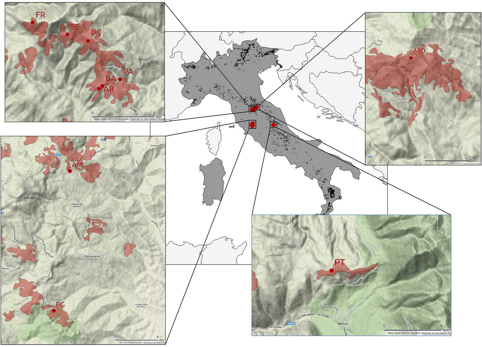
The average density was approximately 2500 trees per hectare following common establishment treatments. Pre-commercial thinning was not applied. No thinning had been carried out at the time of the survey at the following locations: AR, FR, PT, and SC; at the other locations, a light thinning from below was applied. At the time of the survey, stands presented crown closure with ongoing intra-specific competition.
Tab. 2 provides information on the stands from which the trees were selected, such as number of trees, average diameter at 1.3 m height (DBH), DBH range, average height, and height range. The 1098 sampled trees were classified in three social classes: (a) dominant trees (classes 1 and 2 of Kraft - [41]); (b) co-dominant trees (class 3 of Kraft); and (c) subdominant trees (class 4 and 5 of Kraft).
Tab. 2 - Descriptive statistics of the sample trees used for this study.
| Site code | Number of sample trees |
Mean DBH (cm) |
DBH range (cm) |
Mean height (m) |
Height range (m) |
|---|---|---|---|---|---|
| AM | 70 | 23.6 | 14-42 | 22.3 | 18.1-27.5 |
| AR | 85 | 22.9 | 13-34 | 13.6 | 10.4-19.1 |
| BA | 226 | 27.5 | 15-56 | 19.4 | 11.4-27.4 |
| FR | 59 | 30.3 | 18-46 | 19.2 | 14.9-21.8 |
| MO | 137 | 28.7 | 13-51 | 21.3 | 15.6-27.7 |
| PA | 135 | 28.3 | 16-50 | 21.4 | 12.2-26.5 |
| PG | 20 | 33.6 | 26-43 | 24.5 | 21.3-26.8 |
| PS | 102 | 23.2 | 10-38 | 15.2 | 10.1-18.8 |
| PT | 130 | 18.4 | 9-30 | 14.7 | 7.3-19.6 |
| SC | 134 | 24.8 | 13-46 | 20.7 | 14.3-29.0 |
| Total | 1098 | 25.6 | 9-56 | 18.9 | 7.3-29.0 |
The sample trees were selected randomly from each stand. A total of 329 dominant trees, 371 co-dominant trees, and 398 subdominant trees were used for the statistical analysis.
Measures and variables
The tree-level measurements used for the models were: (a) diameter at 1.30 m height (DBH); (b) total height (Ht); (c) height of first living whorl (Hc); (d) projection on the ground of 4 orthogonal crown radii (i.e., North, East, South and West - Rc); and (e) number of living whorls from the top of the crown to the lowest living whorl (LWN).
Five variables, relative to the overall stability of the tree, were selected and included: (a) the number of living whorls (LWN); (b) the height/DBH ratio (slenderness coefficient or taper - HD); (c) the relative depth of the crown (CD); (d) the crown projection (CP); (e) the crown eccentricity (largest radius / smallest radius - EC, [6] - Tab. 3).
Tab. 3 - Descriptive statistics for the following variables: the living whorls number (LWN); the slenderness ratio (HD), the crown depth (CD), the crown projection area (CP) and an eccentricity index of the canopy (EC). (Ht): total height (m); (DBH): diameter at 1.3 m height (m); (Hc): height of first living whorl (m); (Rcmean); arithmetic mean of the crown projection radii (m); (Rcmax): greater of the crown projection radii (m); (Rcmin): smallest of the crown projection radii (m); (CV): coefficient of variation.
| Variable | Dimension | Formula | Min | Mean | Median | Max | CV |
|---|---|---|---|---|---|---|---|
| LWN | count | - | 1 | 16.73 | 16 | 39 | 0.39 |
| HD | adimensional | Ht/DBH | 36.07 | 77.52 | 75 | 148.57 | 0.24 |
| CD | adimensional | 1-(Hc/Ht) | 0.6289 | 35.3891 | 35.4052 | 60.4545 | 0.26 |
| CP | m2 | π Rcmean2 | 0.00014 | 0.379 | 0.36364 | 1 | 0.58 |
| CE | adimensional | Rcmax/Rcmin | 0.126 | 12.788 | 8.042 | 128.648 | 1.19 |
Exploratory analysis
A principal component analysis (PCA) and a non-parametric correlation analysis (NPC) were used to investigate the relationship between the stability indexes (e.g., LWN, HD, CD), and the significant variables were modeled using the Local Weighted Scatterplot Smoothing (LOWESS or LOESS - [11], [12], [13]).
PCA was used to detect the predictability of the five variables (i.e., LWN, HD, CD, CE, CP). The function PRINCOMP {stats} implemented in the R environment ([44]) was applied on the correlation matrix.
The Shapiro-Wilk test ([45]) was used to investigate whether the selected variables were normally distributed (Tab. 4). Significant departures from normality were observed for most variables, as well as for their logarithmic and root square transformation, and therefore a non-parametric statistical analysis was applied. For this reason, the Spearman’s correlation coefficients (ρ - [47]) were calculated to investigate the relationships between the stability indexes and LWN using the function RCORR{Hmisc} of the R software ([23], [44]). Furthermore, the use of a non-parametric test allowed the detection of non-linear relationships among variables.
Tab. 4 - Results of Shapiro-Wilk normality test ([45]).
| Variable Name | Length | W | p-value |
|---|---|---|---|
| LWN | 1098 | 0.9725 | 0.00000 |
| CD | 1098 | 0.9974 | 0.07112 |
| HD | 1098 | 0.9622 | 0.00000 |
| CE | 1028 | 0.9793 | 0.00000 |
| CP | 1028 | 0.6896 | 0.00000 |
| log(LWN) | 1098 | 0.9737 | 0.00000 |
| log(CD) | 1098 | 0.9966 | 0.01689 |
| log(HD) | 1098 | 0.8075 | 0.00000 |
| log(CE) | 1028 | 0.5811 | 0.00000 |
| log(CP) | 1028 | 0.9869 | 0.00000 |
| LWN1/2 | 1098 | 0.9948 | 0.00076 |
| CD1/2 | 1098 | 0.9849 | 0.00000 |
| HD1/2 | 1098 | 0.9714 | 0.00000 |
| CE1/2 | 1028 | 0.9466 | 0.00000 |
| CP1/2 | 1028 | 0.9130 | 0.00000 |
Crown development is influenced by light availability and by the location of each crown in relation to the surrounding trees. For this reason, the correlation test was performed on the whole dataset and by social class. We used a threshold p-level of 0.001 to determine the significance of the correlation coefficients, also considering the Bonferroni’s correction ([18]).
Modeling
The relationship between HD and LWN was modeled using a non-parametric analysis for two reasons: (a) most variables were not normally distributed (Tab. 4) even after logarithmic or square root transformation; (b) LWN is a discrete variable. Moreover, a parametric approach would be not robust because the relationship between the variables was unknown. A Locally Weighted Scatterplot Smoothing regression (LOWESS) was used to this purpose ([11], [12], [13]). The LOESS {stats} function implemented in the R software ([44]) was used to build the model. The portion of the dataset for local smoothing was α = 0.6 with a weight Wi for each decreasing value, as a function of the distance according to the following equation (eqn. 1):
where Di is the distance of the i-th observed value in the α interval; maxDist is the distance of the farthest observed point in the α interval.
To set the α level we performed several attempts, thereby the α level was arbitrarily set at 0.6 under two considerations: (a) lower α levels would introduce undulations in the model due to the local distribution of the data; (b) higher α levels would progressively transform the model towards a linear model.
The local regression was performed by the method of weighted least squares. The analytical form of this non-parametric model was provided by the LOWESS algorithm and applied to data by using an ad-hoc script in R language ([11], [12], [13], [44]). The model was validated by the leave-one-out cross validation using the function ERROREST {ipred} of the R software ([38], [44]). One observation for each of the 1098 model iterations carried out was excluded from the training dataset. Then, the value estimated by the model was compared for each run with the observed value. In this way, the mean square error (RMSE) and the mean square error percentage (% RMSE) were determined.
Results
Significant departures from the normal distribution were observed using the Shapiro-Wilk test for almost all variables and their most common transformations (Tab. 4).
A good correlation both for LWN-CD and LWN-HD was found using the Spearman test (Tab. 5) both for the whole dataset (|ρ| > 0.6) and for all the strata according to the various social classes (|ρ| > 0.45), except for the dominant layer (ρ = 0.33). In both cases, a positive correlation was found between LWN and CD, while a negative correlation was detected between LWN and HD. Furthermore, the correlation coefficient was always highly significant (p < 0.00001). Contrastingly, the correlation between LWN and CE was always poor when using either the entire dataset or the social classes (|ρ| < 0.3). The correlation ceofficient was negative and highly significant (p-value < 0.001). The correlation between LWN and CP was equal to |ρ| = 0.48 when using the whole dataset and decreased to |ρ| <0.3 when the sample was stratified by social class. The correlation was always positive and highly significant (p-value < 0.0001), with the exception of dominant trees.
Tab. 5 - Results of non-parametric correlation tests ([47]) between LWN and the other variables with and without stratification by social classes.
| Stratum | Statistics | CD | HD | EC | CP |
|---|---|---|---|---|---|
| All social classes | ρ | 0.6648 | -0.6263 | -0.2729 | 0.4770 |
| p-value | 0.00000 | 0.00000 | 0.00000 | 0.00000 | |
| Observations | 1098 | 1098 | 1028 | 1028 | |
| Dominant trees | ρ | 0.5357 | -0.3312 | -0.2055 | -0.0981 |
| p-value | 0.00000 | 0.00000 | 0.00026 | 0.08351 | |
| Observations | 329 | 329 | 312 | 312 | |
| Co-dominant trees | ρ | 0.6032 | -0.5226 | -0.1733 | 0.3314 |
| p-value | 0.00000 | 0.00000 | 0.00099 | 0.00000 | |
| Observations | 371 | 371 | 358 | 358 | |
| Sub-dominant trees | ρ | 0.5679 | -0.4763 | -0.0711 | 0.3692 |
| p-value | 0.00000 | 0.00000 | 0.17932 | 0.00000 | |
| Observations | 398 | 398 | 358 | 358 |
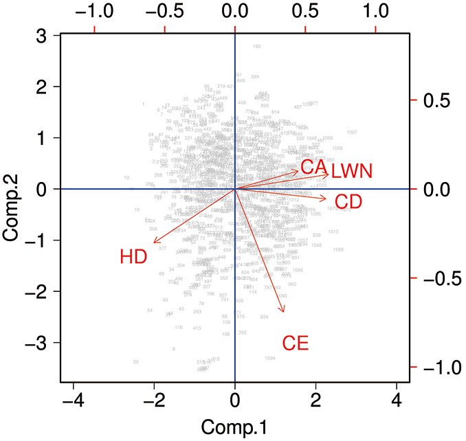
The PCA carried out showed a clear distinction between three groups of variables (Fig. 2). The first group was composed of CP, CD and LWN, the second group was composed of HD and the third group was composed of CE. The first and the second group accounted for a similar amount of variance, but with opposite effect. The third group, instead, was perpendicular to the other two groups and explained an additional portion of the total variance.
Fig. 2 - Biplot of the PCA.
The model obtained for the estimation of the slenderness ratio (HD) based on the based on the living whorls number (LWN) is represented in a graphic form in Fig. 3 and Fig. 4. The leave-one-out cross validation of the local regression model resulted in an accuracy of 82% (RMSE = 14.34, RMSE% = 18%).
Fig. 3 - Model calibration. Model for estimating the slenderness ratio (HD, red line) based on the living whorls number (LWN). Data used for model calibration are plotted (×).
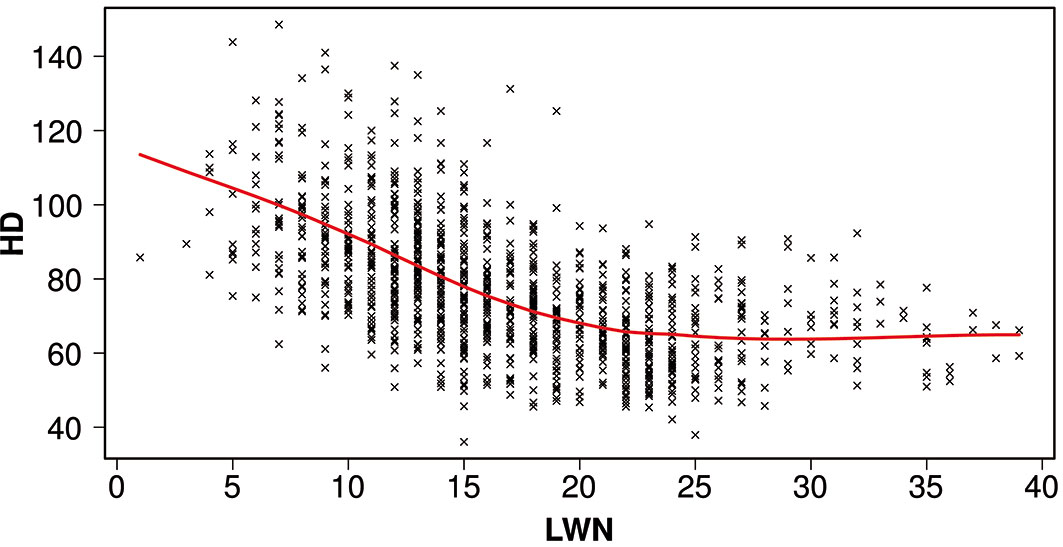
Fig. 4 - Graphical representation of the model obtained (blue line) and its RMSE (light blue area).
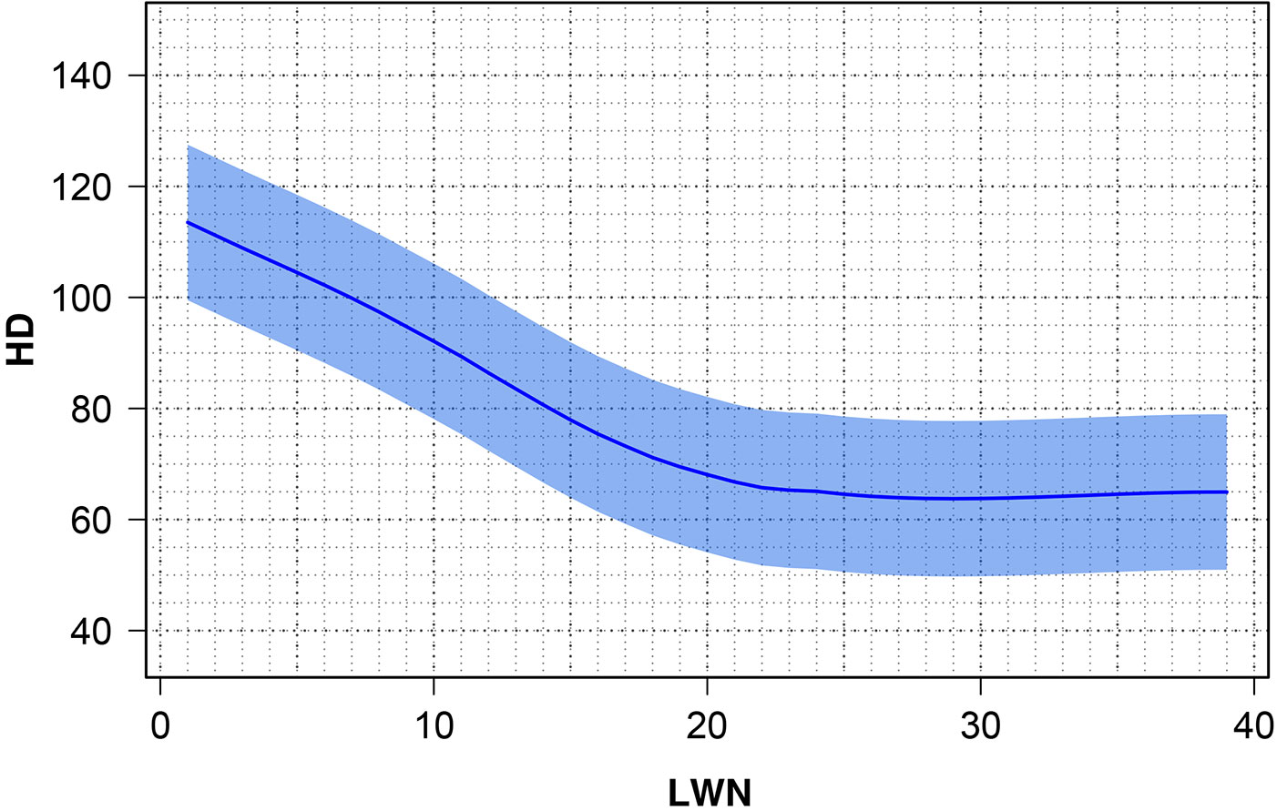
The general form of the model obtained showed a decreasing trend of HD up to a value of LWN = 23. Then, further increases of LWN values did not determine any further reduction of HD.
Discussion and conclusions
The results of this study indicated a significant relationship between LWN and three out of the four selected stability indexes. As expected, the best correlation was recorded between LWN and CD, indicating that the higher is the number of live whorls, the greater is the depth of the crown. This effect may vary according to the distance between whorls. Site fertility and growing conditions have a direct effect of the distance between whorls ([51]), thus site-specific models would increase the predictive ability of LWN.
A significant correlation was also found between LWN and HD. Unlike the previous variables, these two parameters derive from independent measures, which makes LWN a good proxy of the parameter HD. Furthermore, accurate thresholds of stability in terms of HD have been investigated, and therefore LWN may become a valid indicator of individual tree stability.
The relationship between LWN and CP was relatively weak, which is not unexpected. This outcome shows that other factors may affect crown projection. Indeed, crown projection depends strongly on tree density, which was relatively heterogeneous among sites in this study. However, models that include tree density were not a priority, considering that the main goal of the present work was to provide a simple and effective way to assess tree stability in the field.
The relationship between LWN and the eccentricity of the crown was relatively weak though statistically significant. Moreover, modeling by social class did not improve the ability of predicting HD based on the selected variables. The PCA analysis also indicated that HD, LWN, CD and CP indexes were highly correlated. On one hand, this confirms that HD is a strong indicator of tree stability, as suggested by previous studies ([37], [54], [2], [46], [4], [41]). On the other hand, it demonstrates that LWN and CD can be similarly used to explain the same variation of the parameter HD.
In the scientific literature no studies have been carried out specifically about the mechanical stability of the black pine. Instead, many studies have investigated tree stability of European conifers (Tab. 6), including spruce and fir (Picea spp., Abies alba Mill.) and Pinus Radiata D. Don. These studies have indicated that interspecific variability in the HD stability area is relatively low and varies between 75 and 115 (average value = 92.5) for all conifers species combined, while the range is between 85 and 115 (average value = 93.5) for Pinus spp. Compared with other conifers, only larch (Larix decidua Mill.) had a higher tree stability than black pine ([5]). Similar to other conifers, a so-called “HD stability area” is likely between 60 and 90. An HD value above 90 indicates that the pine trees may have stability issues.
Tab. 6 - Reference threshold values of slenderness ratio for the mechanical stability of different conifers.
| Species | Slenderness ratio |
Country of study and additional notes |
Reference |
|---|---|---|---|
| Picea abies (L.) H. Karst | 100 | Germany | Thomasius et al. ([49]) |
| 90 | France - Only for plant from 20 to 30 m of height |
Bequey & Riou-Nivert ([3]) | |
| 100 | Czech republic | Slodicak & Novak ([46]) | |
| 100 | Scotland | Milne ([31]) | |
| 100 | Slovakia | Konôpka ([28]) | |
| 80 | Germany | Abetz ([1]) | |
| Pseudotsuga menziesii Mirb. (Franco) | 75 | Netherlands | Faber & Sissingh ([19]) |
| 85-90 | Italy | La Marca ([29]) | |
| Abies alba Mill. | 85-90 | Italy | La Marca ([29]) |
| Pinus radiata D. Don. | 90-100 | Australia - Only for the largest 200 trees ha-1 | Cremer et al. ([16]) |
| 90 | Galicia | Castedo-Dorado et al. ([10]) | |
| 85 | South Africa | Von Gadow & Bredenkamp ([52]) | |
| 85 | South Africa | Hinze & Wessels ([25]) | |
| Pinus patula Schiede ex Schlechtendal et Chamisso, Pinus elliottii Engelm, Pinus pinaster Aiton, Pinus taeda L. |
115 | South Africa | Hinze & Wessels ([25]) |
| Pinus sylvestris L. | 100 | Scotland | Petty & Swain ([39]) |
| Picea sitchensis (Bong.) Carr. | 85 | United Kingdom | Hamilton & Christie ([22]) |
| Various conifers | 100 | Canada | Wang et al. ([53]) |
In this study, LWN and HD were highly correlated and both showed a strong relationship with tree stability. For all these reasons, our study focused on the relationship between LWN and HD. Furthermore, we demonstrated that there is a constant increase in tree stability for values of LWN up to 23, while for higher values tree stability does not improve even when the number of whorls per tree increases.
Our model provides valid estimates of tree stability for two reasons: (i) the relationship between HD and tree stability indicates a gradual transition around the threshold value from a stable to an unstable tree; (ii) the use of LWN to estimate tree stability indicated that trees can be considered relatively stable for values of LWN higher than 11, and become even more stable for LWN values above 16. This value is conservative and includes the 18% of estimated error. From a forest management perspective, the use of the LWN threshold of 16 may help forest managers to easily select pine trees for thinning. As an example, 50% of trees in our dataset had an LWN value above 16.
In Italy, thinning of black pine forests is usually carried out by selecting trees from below and by using a moderate thinning intensity. In central Italy, the number of trees that can be removed from a stand is restricted by law to 40% of the total. For this reason, thinning carried out on high-density stands may not be able to provide a beneficial effect to the overall stand dynamics, as the remaining trees quickly reach crown closure.
According to the most recent findings, thinning in Italian black pine-dominated forests should be more intense ([9]). The intensity of a thinning-from-below approach should create gaps large enough to allow sufficient light penetration to the understory. Furthermore, we believe that other forest management practices, such as selective thinning, should be encouraged. Black pine is mainly used to reduce land degradation, and selective thinning should aim at maximizing tree health, so that the overall stability of the stand is improved. Released trees should be those more likely to thrive.
Our model provides a useful and easy-to-use tool for selecting the most vigorous trees within a stand based on the number of whorls per tree. Due to the simplified procedure, using LWN to assess tree stability is less time consuming as compared with the use of HD. Indeed, the calculation of HD requires to measure two variables (DBH and Ht), instead of a simple count of the living whorls. This relatively inexpensive method of estimating tree stability can be particularly important because Italian black pine forests have limited financial value, but high ecological and hydrological values.
An additional positive outcome of using LWN to assess tree stability is the easy and feasible quality control of thinning practices by competent authority even after the treatment. This method definitely could be used in operational applications in both private and public black pine stands. Furthermore, similar models also could be developed for other species whose whorls can be easily identified and counted.
References
Gscholar
CrossRef | Gscholar
Gscholar
Gscholar
Gscholar
Gscholar
Gscholar
Online | Gscholar
Gscholar
Gscholar
Gscholar
Gscholar
Authors’ Info
Authors’ Affiliation
Ugo Chiavetta
Consiglio per la Ricerca in Agricoltura e l’Analisi dell’Economia Agraria, Forestry Research Center, v.le Santa Margherita 80, I-52100 Arezzo (Italy)
Corresponding author
Paper Info
Citation
Cantiani P, Chiavetta U (2015). Estimating the mechanical stability of Pinus nigra Arn. using an alternative approach across several plantations in central Italy. iForest 8: 846-852. - doi: 10.3832/ifor1300-007
Academic Editor
Chris Eastaugh
Paper history
Received: Mar 26, 2014
Accepted: Oct 18, 2014
First online: Apr 08, 2015
Publication Date: Dec 01, 2015
Publication Time: 5.73 months
Copyright Information
© SISEF - The Italian Society of Silviculture and Forest Ecology 2015
Open Access
This article is distributed under the terms of the Creative Commons Attribution-Non Commercial 4.0 International (https://creativecommons.org/licenses/by-nc/4.0/), which permits unrestricted use, distribution, and reproduction in any medium, provided you give appropriate credit to the original author(s) and the source, provide a link to the Creative Commons license, and indicate if changes were made.

Web Metrics
Breakdown by View Type
Article Usage
Total Article Views: 51882
(from publication date up to now)
Breakdown by View Type
HTML Page Views: 42487
Abstract Page Views: 3327
PDF Downloads: 4311
Citation/Reference Downloads: 29
XML Downloads: 1728
Web Metrics
Days since publication: 4056
Overall contacts: 51882
Avg. contacts per week: 89.54
Article Citations
Article citations are based on data periodically collected from the Clarivate Web of Science web site
(last update: Mar 2025)
Total number of cites (since 2015): 21
Average cites per year: 1.91
Publication Metrics
by Dimensions ©
Articles citing this article
List of the papers citing this article based on CrossRef Cited-by.
Related Contents
iForest Similar Articles
Research Articles
Estimation of stand crown cover using a generalized crown diameter model: application for the analysis of Portuguese cork oak stands stocking evolution
vol. 9, pp. 437-444 (online: 02 December 2015)
Research Articles
Effect of family, crown position, number of winter buds, fresh weight and the length of needle on rooting ability of Pinus thunbergii Parl. cuttings
vol. 9, pp. 370-374 (online: 11 January 2016)
Research Articles
Fuel characterization and crown fuel load prediction in non-treated Calabrian pine (Pinus brutia Ten.) plantation areas
vol. 15, pp. 458-464 (online: 03 November 2022)
Research Articles
The use of tree crown variables in over-bark diameter and volume prediction models
vol. 7, pp. 132-139 (online: 13 January 2014)
Research Articles
Relationship between tree growth and physical dimensions of Fagus sylvatica crowns assessed from terrestrial laser scanning
vol. 8, pp. 735-742 (online: 11 June 2015)
Research Articles
Predicting tree crown defoliation using color-infrared orthophoto maps
vol. 6, pp. 23-29 (online: 14 January 2013)
Review Papers
Monitoring the effects of air pollution on forest condition in Europe: is crown defoliation an adequate indicator?
vol. 3, pp. 86-88 (online: 15 July 2010)
Research Articles
Estimating crown defoliation of Scots pine (Pinus sylvestris L.) trees using small format digital aerial images
vol. 6, pp. 15-22 (online: 14 January 2013)
Research Articles
Extreme climatic events, biotic interactions and species-specific responses drive tree crown defoliation and mortality in Italian forests
vol. 17, pp. 300-308 (online: 30 September 2024)
Research Articles
Analysing interaction effects in forests using the mark correlation function
vol. 1, pp. 34-38 (online: 28 February 2008)
iForest Database Search
Search By Author
Search By Keyword
Google Scholar Search
Citing Articles
Search By Author
Search By Keywords
PubMed Search
Search By Author
Search By Keyword


