Simplified methods to inventory the current annual increment of forest standing volume
iForest - Biogeosciences and Forestry, Volume 5, Issue 6, Pages 276-282 (2012)
doi: https://doi.org/10.3832/ifor0635-005
Published: Dec 17, 2012 - Copyright © 2012 SISEF
Research Articles
Abstract
The assessment of the current annual increment of forest standing volume (CAI) is a fundamental tool to support forest management and planning. A suitable approach to such an end is to rely on growth and yield models. However, this kind of models are often not available for many countries and/or locations and/or species. Furthermore, they may become obsolete due to potential changes in the environmental and silvicultural conditions. Such shortcomings may be distinctively detrimental in the context of forest inventories. Several methods have been proposed to inventory CAI on one single occasion, i.e., when repeated measurements of standing volume are not available. A well-known family of methods, still largely exploited in Alpine and Eastern European countries, derives from the estimation of the percentage current annual increment of forest standing volume by the current annual increments of stem diameter and tree height (Δh). In this study an experimental comparison of Δh assessment by three different approaches is presented with reference to a properly designed case study: (i) Δh is measured on felled trees; (ii) Δh is estimated by dynamic height curve (i.e., diameter-height-age model); (iii) Δh is estimated by conventional height curve (i.e., diameter-height model). Under the examined experimental conditions (a pure forest of silver fir on highly fertile soils in southern Italy, aged around 60 years), both simplified approaches (ii) and (iii) have proven to underestimate height increments, with a larger underestimation by the approach based on the conventional height curve. However, the consequent error in the estimation of percentage current annual increment of forest standing volume has proved to be quite limited (4% for the approach based on the dynamic height curve and around 9% for the approach based on the conventional height curve). Hence, such simplified approaches may be rather safely considered for estimating percentage current annual increment of forest standing volume when neither Δh is directly detectable on standing trees nor sample trees can be felled, nor an appropriate model to predict Δh is available. The Δh estimation on the conventional height curve should turn out to be even more suitable in the case of uneven-aged stands, where the position of the height curve remains stationary over time.
Keywords
Forest growth, Percentage current annual increment, Current annual increment of tree height, Schneider’s coefficient, Forest management, Forest inventory
Introduction
The assessment of current annual increment of forest standing volume (CAI) is a fundamental tool to support forest management and planning ([2], [7]), in order to quantify the productivity of forest stands, to understand their growth dynamics (at least on a short-term perspective) and to improve the management strategies according to sustainable adaptive approaches.
However, the growth dynamics of a given forest stand is not easy to be reliably assessed on one single occasion, i.e., when repeated measurements of standing volume are not available. A suitable approach to such an end is to rely on growth and yield models (e.g., [27], [10], [21]). However, these kinds of models are often not available for many countries and/or locations and/or species. Furthermore, they may become obsolete due to eventual changes in the environmental and silvicultural conditions ([28]). Such shortcomings may be distinctively detrimental in the context of forest inventories.
Several methods have been proposed for inventorying CAI on one single occasion. A well-known family of methods, still exploited at a large extent in Alpine and eastern European countries, derives from the estimation of the Percentage Current Annual Increment of the forest standing volume (PCAIst). By measuring the forest standing volume of a given stand (Vst), the current annual increment of the stand is then straightforwardly calculated as (eqn. 1):
where (eqn. 2):
where PCAIj is the percentage current annual increment of forest standing volume, referred to the j-th dbh (tree stem diameter at breast height) class; Vj is the forest standing volume, referred to the j-th dbh class; and m is the number of dbh classes in the stand.
All the approaches applied for estimating PCAI are derived from simplifications of the following general formula referred to individual standing trees (eqn. 3):
where Δd is the current annual increment of dbh; d is the dbh; Δh is the current annual increment of tree height; h is the tree height; Δf is the annual variation of tree form factor; f is the tree form factor.
On a short-term perspective, Δf/f is negligible so that the percentage current annual increment of forest standing volume of a given dbh class can be estimated by the assessment of Δdj, Δhj and hj referred to that class (eqn. 4):
Usually, Δd is measured by tree coring at breast height on a representative sample of trees of various dbh classes, so that a relationship between Δd and d can be established, from which Δdj is estimated with reference to the j-th dbh class. Tree height is measured on the same sample of trees on which Δd is measured or on a larger sample, and a relationship between h and d is established (the so-called height curve, known also as diameter-height model), from which hj is estimated with reference to the j-th dbh class. Theoretically, even Δh can be measured on the same sample trees on which Δd is measured, but such attribute is hardly detectable on standing trees (e.g., almost impossible to be detected in the case of mature broadleaved trees), so that the felling of the sampled trees should be required in most cases. When felling a representative sample of trees is impossible (as it happens very often), simplified approaches not requiring the direct mensuration of Δh are adopted.
A suitable approach to such an end is to rely on general models established to predict Δh as a function of easily assessable attributes of standing trees: the models by Stage ([24]) and Hasenauer ([11]) are relevant examples to this respect. However, as previously stressed for growth and yield models, even these particular models are often not available for many countries and/or locations and/or species.
In order to circumvent the estimation of Δh, various practical simplifications of the eqn. 4 are adopted under temperate, alpine and Mediterranean conditions. Distinctively, the simplification proposed by Schneider in 1853 (reported by [22] and [16]) is one of the most commonly adopted in central and southern Europe. To provide growth estimates to forest management, under the so called forest inventory by compartments ([5]), parameters in eqn. 4 are combined into the simpler form ([22], [16] - eqn. 5):
where K is the Schneider’s coefficient and n is the number of tree rings included in the outer centimeter of the core sampled at the breast height.
The parameters n and d can be easily determined by direct measurements in the field. On the other hand, the input of K may become questionable, since the simplicity of the eqn. 5 is more apparent than real. Literature reports the overall range of K values constrained between 400 and 800, with 400 for old-growth trees and 800 for the youngest ones. In practice, the most frequent K values range between 450 and 650 ([12], [13]). However, because of assessment difficulties, it is rather often adopted (e.g., in some Alpine regions) a conventional K value equal to 400 (the so-called K400 criterion, assuming that both Δf/f and Δh/h are negligible) for all the trees sampled in a given forest, with the obvious underestimation of PCAIst. On the other hand, assuming that only Δf/f is negligible (i.e., the same reasonable assumption underlying the eqn. 4), the following formula, derived by equating eqn. 5 with eqn. 4, can be exploited to objectively establish the K value corresponding to a given dbh class when Δh, h and Δd referred to that class are known (eqn. 6):
However, this formula again poses the question of estimating Δh.
Study aim
Simplified approaches for an approximate estimation of the annual increment of tree height in a given forest stand can be exploited when direct mensuration is impossible and general prediction models are not available. A suitable approach is based on the difference between the heights assessed on the height curve (i.e., the diameter-height model established for a given forest stand) with reference to two successive dbh classes and the number of years that a tree takes to move from a given dbh class to the next (i.e., the recruitment period, R) in that stand (eqn. 7):
This approach has been adopted to some extent, e.g., in the Italian National Forest Inventory ([14], [15]). However, the reliability of eqn. 7 for estimating PCAI does not seem to be corroborated yet. In the best of our knowledge, besides Marziliano et al. ([17]), no other peer-reviewed experimental studies have been devoted to this issue: most probably, results concerning this topic are not published nor are they accessible. Such a knowledge gap has stimulated this research note.
The height curve is established on the basis of the sample trees from the stand of interest. However, it is well known that the more an even-aged forest is mature, the more the height curve is flattened ([21]). In such a case tree heights may vary relatively little with increasing dbh. In the case of mature even-aged stands, this suggests that the estimation of Δh through the difference between the heights of two contiguous dbh classes as predicted by the height curve may provide Δh values lower than the actual ones. To circumvent this shortcoming, a so called dynamic height curve (known also as diameter-height-age model), based on the height-dbh relationship as a function of stand age, can be established ([21]).
Here we report the results of a comparison of PCAIst assessment by eqn. 2 and eqn. 4 according to three different approaches for estimating Δh, applied under a properly designed case study: (i) benchmark approach: Δh is measured on felled trees; (ii) dynamic height curve approach: Δh is estimated by the eqn. 7 applied with reference to the dynamic height curve (i.e., the diameter-height-age model); (iii) conventional height curve approach: Δh is estimated by the eqn. 7 applied with reference to the conventional height curve (i.e., the diameter-height model). For further comparison, PCAIst is also estimated by the conventional K400 criterion (i.e., eqn. 5 with a K value equal to 400).
Materials and methods
Field survey
The study site is located within a silver fir (Abies alba Mill.) high forest of approximately 850 hectares, located in the Calabrian Apennines (southern Italy) in the south-west of Serra San Bruno village. The forest is on a plateau at an altitude of about 900 meters a.s.l. characterized by very fertile loamy soils under temperate climate. The stand here observed (“Bosco di Santa Maria”: latitude 38°32’24” N, longitude 16°18’24” E) is on a flat terrain and it is characterized by an even-aged structure including scattered groups of beech trees.
The measurements were carried out in a 0.5 ha plot representative of the average conditions of the stand. The dbh of all the trees with dbh >12.5 cm was measured (Fig. 1). Subsequently, 91 trees (i.e., around 54% of the standing trees) were selected by stratified random sampling, with sample size proportional to the number of trees in each dbh class. An increment core was taken by a Pressler borer at stem breast height on each selected standing tree, on a random direction and perpendicularly to the longitudinal axis of the tree. The total tree height and the height increments corresponding to the last ten years were measured on the same selected trees just after the felling. Tab. 1 summarizes the main descriptive statistics of the measured dendrometrical parameters, all of which show normality of distribution.
Fig. 1 - Tree dbh distribution in the examined stand.
Tab. 1 - Descriptive statistics of the attributes measured on the sampled trees. (SD): standard deviation; (SE): standard error.
| Attribute | mean | SD | Skewness | Skewness SE |
Kurtosis | Kurtosis SE |
|---|---|---|---|---|---|---|
| dbh (cm) | 37.4 | 11.3 | 0.85 | 0.25 | 0.91 | 0.50 |
| current annual increment of dbh (cm yr-1) |
0.60 | 0.12 | 0.37 | 0.25 | -0.61 | 0.50 |
| height (m) | 26.9 | 3.41 | 0.05 | 0.25 | -0.05 | 0.50 |
| current annual increment of height (m yr-1) |
0.28 | 0.07 | -0.06 | 0.25 | -0.40 | 0.50 |
Lab analyses and data processing
Fig. 2 - Current annual increment of dbh vs. dbh from the sampled trees, with the established functional relationship superimposed.
Annual stem growth ring count and width measurement (with a precision of 1/100 mm) were carried out on the last ten rings of each sampled core by the LINTAB system (RinnTec) associated with TSAP software (⇒ http://www.rinntech.de/content/view/16/47/lang,english/). Δd was calculated as 2·r10/10 where r10 is the increment of the radius occurred in the last 10 years. The Δd-d relationship was then established on the sampled trees, taking care of subtracting the measured Δd value (expressed in cm yr-1) to the d value (expressed in cm) measured on the same tree. Among various functional forms, the semilogarithmic one proved to be the most suitable (Fig. 2 - eqn. 8):
with R2 = 0.67 and SEE = 0.071 cm yr-1. The recruitment period, i.e., the number of years that a tree of average size takes to move from a dbh class to the next (according to a dbh class width equal to 5 cm), is given by Rj = 5/Δdj, where Δdj is the current annual dbh increment predicted by the eqn. 8 for the j-th dbh class.
Fig. 3 - Current annual increment of tree height vs. tree height from the sampled trees, with the established functional relationship superimposed.
Δh was calculated as Δh = l10/10, where l10 is the stem length corresponding to the height increment in the last 10 years. The Δh-h relationship was established on the sampled trees, taking care of subtracting the measured Δh value (expressed in m yr-1) to the h value (expressed in m) measured on the same tree. Among various functional forms, the linear one proved to be the most suitable (Fig. 3 - eqn. 9):
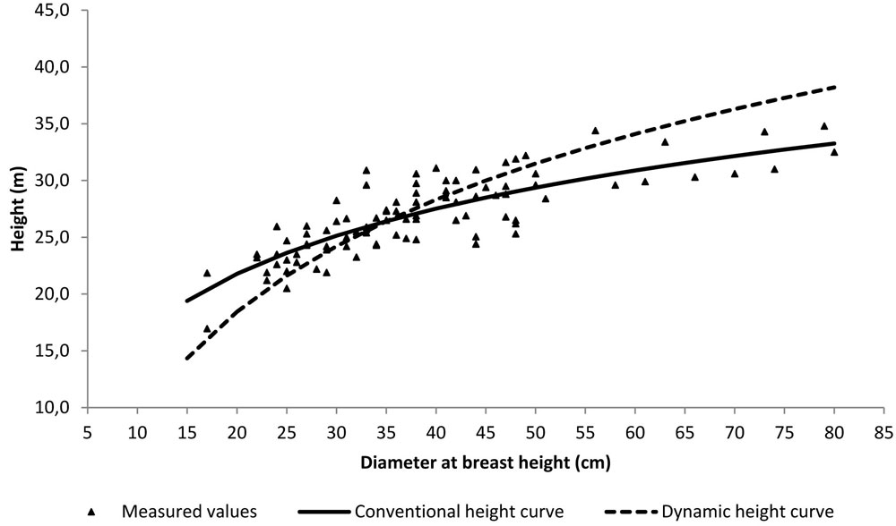
with R2 = 0.59 and SEE = 0.05 m yr-1. The conventional height curve was established by the scatterplot of the heights vs. dbh values measured on the sampled trees. As suggested by Hellrigl ([13]), the dynamic height curve was established by the scatterplot of the heights vs. dbh values corresponding to the average-size tree predicted for each age class by the local yield table for Abies alba stands, first fertility class ([20]), provided that stand density and mean height of the examined stand was comparable with those reported for this fertility class at the same age. Fig. 4 shows the scatterplot of the height vs. dbh values measured in the considered stand, with both the conventional and the dynamic height curves superimposed: as expected, the dynamic curve is much steeper than the conventional one, since it explicitly takes into account height growth dynamics.
Fig. 4 - Scatter-plot of measured height vs. dbh values from the sampled trees, with the conventional and the dynamic height curves superimposed.
PCAIj was estimated by eqn. 4 for the approaches (i), (ii) and (iii) mentioned in the chapter “Study aim”, while it was estimated by eqn. 5 for the application of the K400 criterion (where nj = 2/Δdj) ). For all cases Δdj was obtained by eqn. 8 and h was obtained by the conventional height curve. Δhj was obtained either directly applying eqn. 9 in the case of the benchmark approach or by applying eqn. 7 in the cases of the dynamic and the conventional height curves. The standing volume was estimated by the Italian National Forest Inventory volume models valid for silver fir ([26]).
Results
At the time of inventory, the average tree age was about 60 years; the number of trees per hectare was 336; beech was present with 40 individuals per hectare, i.e., 12% of the total of trees. The distribution of trees by dbh classes showed a typical bell-shaped pattern, with dbh up to 80 cm (Fig. 1) and a quadratic mean dbh (qmd) of silver fir around 44 cm. The tree height corresponding to qmd was around 28 m; the wood volume of the trees with dbh>12.5 cm was 651 m3 ha-1, of which 93% was due to the silver fir.
The examined stand is characterized by Δd ranging from 0.36 to 0.41 cm yr-1 for the smallest dbh class (15 cm) and from 0.80 to 0.89 cm yr-1 for the largest one (80 cm). Correspondingly, the period for a tree of a given dbh class to move onto the next dbh class ranges, on average, from 16 years for the 15-cm dbh class down to 6 years for the 80-cm dbh class. Measured Δh ranges from 0.40 to 0.45 m yr-1 for the smallest dbh classes and from 0.15 to 0.21 m yr-1 for the largest ones (31-35 m).
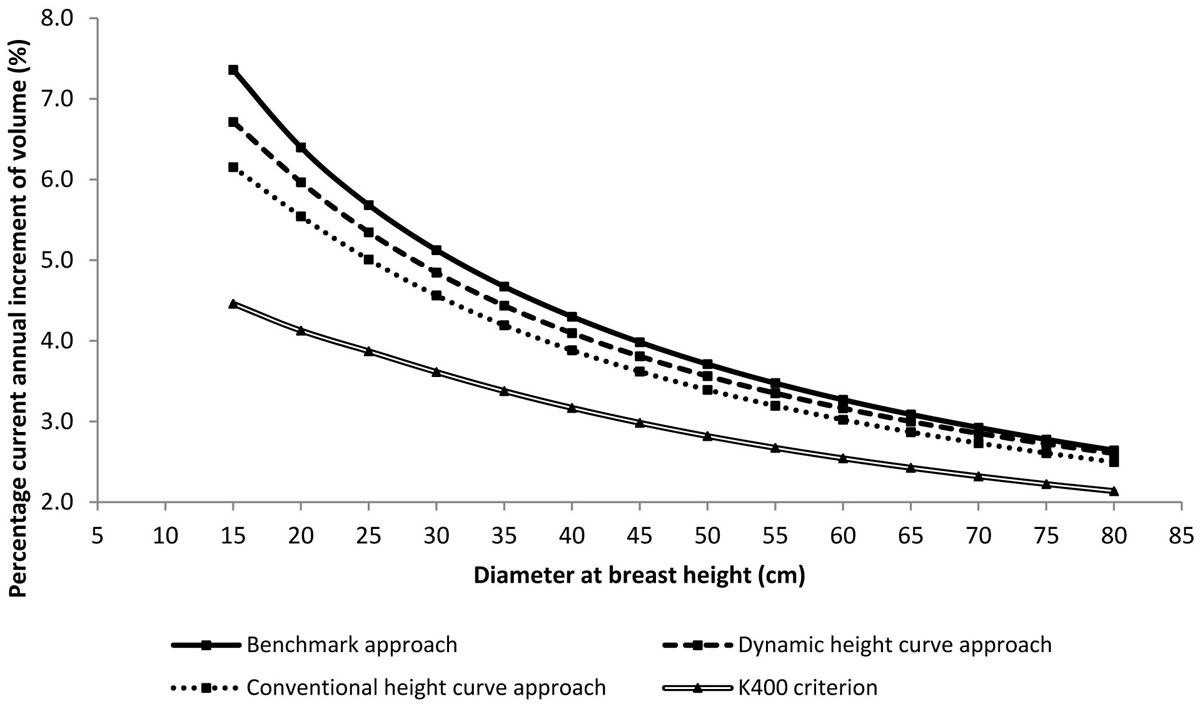
Tab. 2 shows the high significance (p<0.01, according to the paired-sample t test and to the Wilkoxon paired-sample test - [29]) of the Δh estimation differences between the simplified and the benchmark approaches. Fig. 5 shows the PCAIj values estimated for each dbh class by the three compared approaches and by the K400 criterion. As expected, PCAIj decreases with increasing dbh. Both simplified approaches adopted to assess Δh do underestimate PCAIj, for all the dbh classes as per the approach based on the conventional height curve and for the classes below 60-65 cm as per the approach based on the dynamic height curve. The differences between the simplified approaches and the benchmark approach are larger for the smaller dbh classes and become smaller for the larger ones. Distinctively, PCAIj ranges from 7.4% with respect to the 15-cm dbh class down to 2.6% with respect to the 80-cm dbh class for the benchmark approach, while it varies, respectively, from 6.7% to 2.6% according to the dynamic height curve approach and from 6.2% to 2.5% according to the conventional height curve approach. The percentage current annual increment of forest volume at stand level is equal to 3.8% for the benchmak approach, to 3.6% for the dynamic height curve approach, and to 3.4% for the conventional height curve approach. Hence, the dynamic height curve approach gives smaller differences (less than half) than the conventional one as to the benchmark. Distinctively, the PCAIst assessment by the dynamic height curve approach can be considered fairly accurate. On the contrary, the K400 criterion brings to a relevant underestimation of PCAIst (2.7%).
Tab. 2 - Significance of the Δh estimation differences between the simplified and the benchmark approaches, assessed by the paired-sample t test (T) and to the Wilkoxon paired-sample test (Z) for the dbh classes in the examined stand.
| Paired comparison | T | Z |
|---|---|---|
| dynamic height curve approach - benchmark approach |
7.07 (p<0.01) |
-3.30 (p<0.01) |
| conventional height curve approach - benchmark approach |
9.38 (p<0.01) |
-3.30 (p<0.01) |
Fig. 5 - Trends of percentage current annual increment of volume calculated in the examined stand according to the three approaches compared for assessing Δh and to the K400 criterion.
The CAI values assessed by eqn. 1 range from 22.8 m3 ha-1 yr-1 for the benchmark approach to 21.9 m3 ha-1 yr-1 for the dynamic height curve approach, to 20.8 m3 ha-1 yr-1 for the conventional height curve approach and to 16.5 m3 ha-1 yr-1 for the K400 approach. As expected, similarly to what observed for the Δh estimation differences, even the differences among the CAI values obtained by the three compared approaches and the K400 criterion (Tab. 3) are significant (p<0.01), according to the paired-sample t test and to the Wilkoxon paired-sample test. The CAI shows its maximum value with reference to the 50-cm dbh class, with a value of 3.8 m3 ha-1 yr-1 for the benchmark approach, a value of 3.6 m3 ha-1 yr-1 for the dynamic height curve approach, a value of 3.5 m3 ha-1 yr-1 for the conventional height curve approach and a value of 2.9 m3 ha-1 yr-1 for the K400 criterion.
Tab. 3 - CAI values estimated for each dbh class in the examined stand by the compared approaches.
| dbh class (cm) |
Benchmark approach for assessing Δh (m3 ha-1 yr-1) |
Dynamic height curve approach for assessing Δh (m3 ha-1 yr-1) |
Conventional height curve approach for assessing Δh (m3 ha-1 yr-1) |
K400 criterion (m3 ha-1 yr-1) |
|---|---|---|---|---|
| 15 | 0.14 | 0.13 | 0.11 | 0.08 |
| 20 | 0.33 | 0.30 | 0.28 | 0.21 |
| 25 | 0.62 | 0.59 | 0.55 | 0.42 |
| 30 | 1.04 | 0.99 | 0.93 | 0.74 |
| 35 | 1.71 | 1.62 | 1.53 | 1.24 |
| 40 | 3.12 | 2.98 | 2.82 | 2.30 |
| 45 | 3.34 | 3.19 | 3.04 | 2.50 |
| 50 | 3.80 | 3.65 | 3.47 | 2.89 |
| 55 | 3.05 | 2.94 | 2.81 | 2.35 |
| 60 | 1.90 | 1.84 | 1.76 | 1.48 |
| 65 | 1.85 | 1.80 | 1.72 | 1.46 |
| 70 | 1.04 | 1.02 | 0.98 | 0.83 |
| 75 | 0.39 | 0.38 | 0.36 | 0.31 |
| 80 | 0.43 | 0.42 | 0.41 | 0.35 |
Tab. 4 shows the K values obtained from eqn. 6 for each dbh class of the examined stand, according to the three different approaches used to assess Δh. High K values are characteristics of trees with a high relative height increment and a low relative dbh increment, as it usually happens for the smallest dbh classes within a given stand, while the opposite usually holds for the largest ones: consequently, K tends to decrease with increasing dbh. As a result, K significantly decreases from 688 for the 15-cm dbh class down to 495 for the 80-cm dbh class (values referred to the benchmark approach for assessing Δh). Similarly to PCAIj, the approach based on the dynamic height curve underestimates the Kj values up to dbh of 75 cm, while the conventional height curve approach underestimates the Kj values for all the dbh classes and provides K values more different from that of the benchmark approach than those provided by the dynamic curve approach. The differences of the estimated K values among the approaches used here to assess Δh are higher for the smallest dbh classes and become smaller with an increasing dbh.
Tab. 4 - Schneider’s coefficient K obtained from eqn. 6 according to the three different approaches for assessing Δh.
| dbh class (cm) |
Benchmark approach |
Dynamic height curve approach |
Conventional height curve approach |
|---|---|---|---|
| 15 | 688 | 628 | 575 |
| 20 | 620 | 578 | 537 |
| 25 | 587 | 553 | 518 |
| 30 | 567 | 537 | 505 |
| 35 | 553 | 525 | 497 |
| 40 | 543 | 517 | 490 |
| 45 | 534 | 511 | 485 |
| 50 | 527 | 506 | 481 |
| 55 | 520 | 501 | 478 |
| 60 | 514 | 498 | 475 |
| 65 | 509 | 495 | 473 |
| 70 | 504 | 492 | 471 |
| 75 | 499 | 490 | 469 |
| 80 | 495 | 488 | 467 |
Discussion
In this study, two simplified approaches to assess the current annual height increment within the framework of the estimation of PCAI have been tested in an even-aged stand. Under the examined conditions, both simplified approaches have proven to underestimate height increments, with a larger underestimation by the approach based on the conventional height curve. However, the consequent error in the estimation of PCAI is quite limited (4% for the approach based on the dynamic height curve and around 9% for the approach based on the conventional height curve), relative to the benchmark approach. Hence, such simplified approaches may be rather safely considered for estimating PCAI when neither Δh is measureable on standing trees nor sample trees can be felled nor an appropriate model to predict Δh is available.
Theoretically, both the simplified approaches are relatively easy to be implemented. However, the dynamic height curve approach is applicable only when an established diameter-height-age model is available and valid for the stand of interest, or when stands of various ages with composition, site fertility and silvicultural treatment similar to those of the stand of interest are available.
Alternatively, the approach based on the conventional height curve can be applied: in this case, underestimation as broad as 9% may be expected as concerns the assessment of the PCAI in even-aged stands under conditions like those examined in this study. On the other hand, it can be straightforwardly evidenced that to neglect Δh/h in eqn. 4, as e.g., carried out in the professional practice by adopting the so-called K400 criterion (see the chapter “Introduction”), conveys too large underestimation, e.g., an unaffordable CAIst underestimation of nearly 1/3 in the examined case study. In the light of this, when no other practical tools are available, the Δh estimation obtainable from eqn. 7 on the conventional height curve is still an advisable option. Furthermore, this tool should be even more suitable in the case of uneven-aged stands, where the position of the height curve remains stationary over time (i.e., the height growth in the individual dbh classes remains almost constant, see [21]).
Further considerations can be drawn from the test carried out. From a general point of view, longitudinal and radial stem growth show different patterns ([25]): under natural conditions, a decrease of the longitudinal growth with size can be observed for most tree species, while radial growth tends to be constant for long time ([9]). Although age influence cannot be completely excluded, various authors (e.g., Maggs 1964 in [8], [18], [1], [19]) have shown that the reduction of height increment is mainly due to functional tree-size constraints: from a practical point of view, small trees tend to have greater relative height increments regardless of age, while large trees tend to have gradually smaller relative ones. Thus, the chronological rule-of-thumb proposed by Müller in 1915 and reported by la Marca ([16]), and widely adopted by professionals in practical forest management (at least in Italy and in the Alpine region), by which the tree age is the driver of the relationship between Δh/h and Δd/d, may be misleading. By such a rule, the Schneider’s coefficient K is conventionally set equal to around 400 for old trees (i.e., Δh/h = 0), to around 600 for mature trees (i.e., Δh/h = Δd/d) and to around 800 for young trees (i.e., Δh/h = 2 · Δd/d), and analogous K reference values are adopted for assessing PCAI of entire even-aged stands. From a trivial point of view, it might seem obvious to associate size with age (especially as concerns the animals), but this is not invariably true for forest trees ([23]), where old small individuals, and vice-versa trees with huge biomass accumulated in few decades, can be found. Then, it is advisable that K values are correctly assigned in the practice not with reference to the age (i.e., as prescribed by the above mentioned chronological rule-of-thumb), but with reference to the size of the trees. Actually, this suggestion is corroborated by the test presented here, where trees of the same age were characterized by very different K values, according to their dbh class (Tab. 4). eqn. 6 and the connected approaches for estimating Δh are helpful tools for pinpointing the suitable K values.
Conclusion
As a matter of fact, objective decisions need objective information ([4]). Only a sufficiently accurate assessment of forest growth can effectively support management and planning: a suitable silvicultural treatment cannot be properly devised if stand volume increment is not assessed with enough detail, at least on a short-term perspective, along with tree density, composition, stand structure and volume. This issue is distinctively relevant under an updated vision of forestry, to move from a strictly ruled forest planning to adaptive management, where reliable and cost-efficient monitoring tools become mandatory ([6]).
Within this framework, the eqns. 2, 4 and 7 are suitable for assessing the percentage current annual increment of forest standing volume within sample plots under practical forest inventory purposes on a single occasion, both on a stand-wise level (forest inventory by compartments) or within assessments at larger scales. The simplicity of such formulas is attractive, though they are characterized by several limitations: for instance, the procedure does not take into account tree mortality. However, it gives reasonable predictions on a short-term perspective, when tree mortality can be neglected, leading to a suitable assessment of the current productivity of the considered forest stands. Obviously, the obtained figures are relative to the stands measured and cannot be extrapolated for long periods or to other stands: in this respect, only proper growth and yield models should be exploited (for reference, e.g. [27], [10], [3], [21], [28]).
As for eqn. 7, whose previously unknown reliability has been the main motivation of this work, it may be safely applied under conditions like those examined here for quantifying the value of Δh when neither this parameter is directly measurable on standing trees nor sample trees can be felled nor appropriate prediction models are available. In the light of this, the effectiveness of such an approach is worth to deserve further investigation under various compositional, structural and silvicultural conditions.
Acknowledgments
This study was partially developed within the scope of research project “FUME - Forest fires under climate, social and economic changes in Europe, the Mediterranean and other fire-affected areas of the world”, European Commission FP7-ENV-2009, Grant Agreement Number 243888.
We thank the company “La Foresta s.r.l. di Serra San Bruno” for the willingness shown during the surveys in the field.
We also thank four anonymous reviewers for their helpful suggestions on an earlier draft of this paper.
References
Gscholar
Gscholar
Gscholar
Gscholar
Gscholar
Gscholar
Gscholar
Gscholar
Gscholar
Gscholar
Gscholar
Gscholar
Gscholar
Gscholar
Gscholar
Gscholar
Gscholar
Authors’ Info
Authors’ Affiliation
G Menguzzato
A Scuderi
Dipartimento di Gestione dei Sistemi Agrari e Forestali (GESAF), Mediterranean University di Reggio Calabria, Loc. Feo di Vito, I-89060 Reggio Calabria (Italy)
Dipartimento per l’Innovazione nei sistemi Biologici, Agroalimentari e Forestali (DIBAF), University of Tuscia, v, San Camillo de Lellis snc, I-01100 Viterbo (Italy)
Corresponding author
Paper Info
Citation
Marziliano PA, Menguzzato G, Scuderi A, Corona P (2012). Simplified methods to inventory the current annual increment of forest standing volume. iForest 5: 276-282. - doi: 10.3832/ifor0635-005
Academic Editor
Marco Borghetti
Paper history
Received: Jul 18, 2012
Accepted: Oct 16, 2012
First online: Dec 17, 2012
Publication Date: Dec 28, 2012
Publication Time: 2.07 months
Copyright Information
© SISEF - The Italian Society of Silviculture and Forest Ecology 2012
Open Access
This article is distributed under the terms of the Creative Commons Attribution-Non Commercial 4.0 International (https://creativecommons.org/licenses/by-nc/4.0/), which permits unrestricted use, distribution, and reproduction in any medium, provided you give appropriate credit to the original author(s) and the source, provide a link to the Creative Commons license, and indicate if changes were made.

Web Metrics
Breakdown by View Type
Article Usage
Total Article Views: 49796
(from publication date up to now)
Breakdown by View Type
HTML Page Views: 42236
Abstract Page Views: 2321
PDF Downloads: 3826
Citation/Reference Downloads: 74
XML Downloads: 1339
Web Metrics
Days since publication: 4148
Overall contacts: 49796
Avg. contacts per week: 84.03
Article Citations
Article citations are based on data periodically collected from the Clarivate Web of Science web site
(last update: Feb 2023)
Total number of cites (since 2012): 19
Average cites per year: 1.58
Publication Metrics
by Dimensions ©
Articles citing this article
List of the papers citing this article based on CrossRef Cited-by.
Related Contents
iForest Similar Articles
Research Articles
Scots pine’s capacity to adapt to climate change in hemi-boreal forests in relation to dominating tree increment and site condition
vol. 14, pp. 473-482 (online: 18 October 2021)
Commentaries & Perspectives
Benefits of a strategic national forest inventory to science and society: the USDA Forest Service Forest Inventory and Analysis program
vol. 1, pp. 81-85 (online: 28 February 2008)
Review Papers
Integration of forest mapping and inventory to support forest management
vol. 3, pp. 59-64 (online: 17 May 2010)
Commentaries & Perspectives
Reply: “Use of BIOME-BGC to simulate Mediterranean forest carbon stocks”
vol. 4, pp. 249 (online: 03 November 2011)
Research Articles
Genetic control of intra-annual height growth in 6-year-old Norway spruce progenies in Latvia
vol. 12, pp. 214-219 (online: 25 April 2019)
Research Articles
Using self-organizing maps in the visualization and analysis of forest inventory
vol. 5, pp. 216-223 (online: 02 October 2012)
Research Articles
Relationship between tree growth and physical dimensions of Fagus sylvatica crowns assessed from terrestrial laser scanning
vol. 8, pp. 735-742 (online: 11 June 2015)
Research Articles
Allometric models for the estimation of foliage area and biomass from stem metrics in black locust
vol. 15, pp. 281-288 (online: 27 July 2022)
Technical Advances
Improved estimates of per-plot basal area from angle count inventories
vol. 7, pp. 178-185 (online: 17 February 2014)
Research Articles
Effects of defoliation by the pine processionary moth Thaumetopoea pityocampa on biomass growth of young stands of Pinus pinaster in northern Portugal
vol. 3, pp. 159-162 (online: 15 November 2010)
iForest Database Search
Google Scholar Search
Citing Articles
Search By Author
Search By Keywords


