Introduction 

Thermodynamic methods for measuring sap flow are widely used in forestry, hydrology, agronomy and eco-physiological studies to accurately estimate tree water use, to identify specific drought stress conditions or to understand plant functionality. These methods which depend on heat transfer, however, differ fairly widely in their capabilities and limitations, notably in their sensitivity to low, zero and reverse flow rates. Reverse sap flow is particularly important for understanding the whole plant physiology and tree architecture, and acts as an indicator of hydraulic redistribution ([22], [24], [4], [33]). In thermodynamic methods, thermometers are commonly used to gauge temperature changes of the heat field around a heater in response to sap movement. Thermometers may be arranged around the heater either symmetrically or asymmetrically. For symmetrical measurements, they are placed above and below and at equal distance from the heater in the axial direction ([10], [46], [37], [41], [19], [21], [22], [5]), while for asymmetrical measurements, the above thermometer is substituted by one placed together with the heater. ([15], [6], [12]).

The majority of methods using thermometers arranged symmetrically around a heater produce accurate sap flow measurement with good dynamic resolution with the true sap flow under low flow conditions ([46], [17], [36], [22]). The situation can be different, however, under high flow rate conditions when a symmetrical sensor output does not correlate linearly with flow rates and renders a diurnal variation with two peaks, corresponding to one in the morning and one in the afternoon, with a drop at around midday (e.g., [15] in spruce, [41] in pine, [20], [22] in apple). This type of curve was called later “a McDonalds curve” ([1]). This particularity or “disadvantage” associated with measuring symmetrical temperature difference also known as sap flow index (SFI) proved in fact to be very useful for the purpose of irrigation control, and as a reliable indicator of water stress and water storage use ([19], [22], [23], [35]). Methods which use asymmetrical arrangements of thermometers are well suited for measuring medium and high flow rates, but they are problematic for measuring low flow rates to accurately distinguish zero flow. Another disadvantage of these methods is that they cannot measure bi-directional flows.

The Heat Field Deformation (HFD) technique is one of thermodynamic methods for measuring sap flow. It uses a continuous linear heating system thus enabling high time resolution measurements, which are important for studies on plant responses to abrupt environmental changes ([9], [27]). The HFD technique combines the most advantageous features of previously developed methods by measuring both asymmetrical and symmetrical temperature gradients, dT_sym and dT_as, around a heat source, and avoids the limitations associated with thermometer arrangement previously applied separately. Furthermore, the sensor configuration using the HFD method involves placing the upper thermometer of the asymmetrical thermocouple next to a heater, which for the first time makes it possible to follow heat dissipation and deformation in both axial and tangential directions around a linear heater. This configuration has also been applied later to the impulse sap flow technique ([44]). Since the HFD technique was first developed by Nadezhdina in 1991, this methodology has been generally described in several works ([25], [28], [29], [30], [34]). At the heart of this methodology is the anaysis of variation of temperature differences around a linear heater using a K-diagram. To date, only two literature sources have partially addressed this key concept ([28], [25]). The aim of this work is to offer a more comprehensive description of how K-diagrams are used to analyze measured temperature differences and correctly determine K-values, which are critical for accurately calculating sap flow from the measured temperature records and for interpreting the results.

  Sensor design and configuration 

The Heat Field Deformation (HFD) method was originally developed for sap flow measurements in tree organs with diameters larger than 3 cm. The sensor configuration includes the needle-like heater radially inserted in the sapwood and two pairs of differential copper-constantan thermocouples, whose lower reference thermometers are inserted in one common needle for both differential thermocouples and placed below a heater. The displacement of needles with thermometers drives the geometric shape of a heat field around a heater under zero flow conditions (Fig. S1 and Fig. S2 in Supplementary material). In the symmetrical pair of thermocouples, the thermometers are positioned equidistantly from the heater in the axial direction at distance Z_sym from each other (twice the distance of each thermometer from the heater, Z_ax), and measure dT_sym allowing for bi-directional (acropetal and basipetal) and very low flow measurements ([21], [22]). In the asymmetrical pair of differential thermocouples, the upper portion is removed from the heater in the tangential direction at distance Z_tg. This pair of thermocouples, measuring dT_as is mostly responsible for gauging the magnitude of medium and high sap flow rates. This applied configuration of thermometers allows for calculations of the third temperature difference dT_s-a as being the difference between dT_sym and dT_as.

ICT International (Armidale, Australia) developed a more technologically advanced version of the HFD sensor using the same original configuration, but where the needles contain equidistantly placed thermistors (instead of thermocouples) and where needles are connected to a 24-bit digital microprocessor-based smart interface (⇒ http:/­/­www/­ict.­international). The advantages of the ICT-modified HFD technique is that it represents a stand-alone system with an integrated logger and battery allowing for wireless connectivity and data transfer.

Beyond the classical configuration of the HFD sensor, several modifications for sap flow measurements in plant stems lower than 2 cm in diameter were tested. Designs of Baby HFD sensors with external (exo-sensors) and internal (endo-sensors) heating and examples of their applications are described in Nadezhdina ([26]). For all types of Baby HFD sensors the same original principle is used: the ratio of measured temperature differences around a heater is taken as a measure of sap flow. The application of the same method in all sizes of trees and their organs may increase an accuracy and reliability of comparable tree water relation studies. Recently the exo-sensors were effectively applied in such small plant organs as tomato peduncle ([13]) and truss ([14]).

3D dimension of the HFD method

An important step for verifying the HFD methodology was conducting sap flow measurements in the stem of a Tilia cordata tree while simultaneously monitoring changes to the heat field generated by the heater of the HFD sensor using an infrared radiation (IR) camera. These experiments were conducted at the Hahn-Meitner Institute in Berlin in 1998 and the results were published in several papers ([29], [42], [43]). I will use several IR images of these real heat fields throughout this text to further illustrate the HFD methodology.

IR imaging provides a salient three-dimensional visualization of the HFD method. Tangential and radial views of the heat field generated around a linear heater are shown in Fig. S1 (Supplementary material), both under conditions of zero flow and ascending sap. A tangential view of the heat field demonstrates two dimensions: axial and tangential which differ even for conditions of zero flow (Fig. S1c), as thermal conductivity is higher in the axial than in the tangential direction. The anisotropy of sapwood produces a heat field in a symmetrical ellipse form under zero flow (whereas in an isotropic medium, the heat field would be in the form of a circle). Moving sap deforms the elliptical heat field in the tangential stem section (Fig. S1d) as well as in a radial direction along sapwood depth, where water movement occurred (Fig. S1f). This illustrates that the assumption of a perfect linear heater with equal temperature ([45]) can, in reality, only be valid under zero flow (Fig. S1e). Under moving sap conditions, the temperature of a heater cannot be radially even as more heat is stored in the heartwood (shown as the hottest area in Fig. S1f), whereas the coldest zone in a heater occurs in sapwood depths with the highest flow rates. Effectively, a radial view of a heat field near the same heater will differ for trees with different proportions of sapwood and heartwood depths. Combining radial and tangential views of the heat field near a linear heater under moving sap conditions makes it possible to visualize the HFD method as a 3D image (Fig. S2 in Supplementary material).

  K-diagram - the relationship between measured temperature differences and their ratio 

It has been empirically proven that the dT_sym/dT_as ratio is proportional to sap flow rates ([28], [25]). Analysing the relationship between temperature differences around a linear heater and the dT_sym/dT_as ratio (Fig. 1) represents a core concept in the HFD method. This relationship is referred to as what is called a “K- diagram”, which is particularly well suited to determining K-value. K-value is the value of dT_as or dT_s-a for a zero flow condition, when these two temperature differences are equal to each other in absolute values and when dT_sym (thus, also the dT_sym/dT_as ratio) are equal to zero. Thus, for zero flow conditions K-values can be easy determined as intersection of dT_as or dT_s-a with Y axis of a K-diagram.

Fig. 1 - Relationships between temperature differences and their ratios constructed for a Quercus suber tree. (a): K-diagram - relationship between temperature differences dT_sym, dT_as, dT_s-a and the ratio dT_sym /dT_as. One day (24 hours) of records is presented with maximum values for dT_sym /dT_as corresponding to maximum daily flow rates. Each temperature difference has a daily loop with higher values in the morning and lower values in the evening. K is equal to 1.7 °C. Arrow indicate the alignment of daily records of dT_sym by using (K+dT_s-a) instead of it. (b): K/R-diagram - relationship between the temperature differences (K+dT_s-a) and dT_as and their ratio (K+dT_s-a)/dT_as. The asymmetrical temperature difference is presented here as the ratio 1/dT_as using the second Y-axis for the better illustration of the HFD principle. Blue and red ellipses demonstrates “active” and “inactive” parts of each temperature curves in the calculation of sap flow, which is proportional to the ratio (K+dT_s-a)/dT_as.

  Enlarge/Shrink   Download   Full Width  Open in Viewer

K-diagrams are also useful for explaining the analysis at the heart of the HFD method: using independent readings indicating the sensitivity of measured temperature gradients, and alternating them out (switching) when one gradient becomes non-sensitive. The maximum levels for both dT_as and dT_sym serve as threshold values, where the switching between the sensitivity of the measured temperature gradients takes place. This transition zone is rather narrow for most species. Ideally, dT_sym should be constant and should not decrease after approaching its maximum value, which is never the case in real conditions. It was found that both temperature gradients, dT_sym and dT_s-a, are directly and highly proportional under very low flow rates up to their maximum value and they differ between each other on K- value (Fig. 1a). Additionally, dT_s-a remains almost constant with further progressively increasing flow rates, whereas dT_sym begins to decrease after reaching its maximum value in the morning (Fig. 1a). Given this dynamic, it was suggested that the new temperature difference (K+dT_s-a) should be used to substitute dT_sym in sap flow calculation. To illustrate the HFD method in clearer terms, Fig. 1b, where the second Y-axis was applied for the 1/dT_as ratio instead of dT_as, shows the alternating importance of both temperature gradients under changing flow rates: (K+dT_s-a) is “active” under low flow, whereas 1/dT_as starts to be sensitive once further flow increases after passing the transition zone. From this point forward, (K+dT_s-a) became constant. It is important here that for the whole range of variable ratios (K+dT_s-a)/dT_as, when one temperature gradient changes, the second remains unchanged and has no apparent influence on flow calculation. In this way, the advantages of both thermocouple arrangements around a linear heater can be exploited without the limitations occurring when each of them are used separately.

From the example of single day records of temperature gradients shown via the K-diagram and presented in Fig. 1a, we can see that only two temperature gradients, dT_as and dT_s-a, are essential for K-value determination. Two other temperature gradients, dT_sym and (K+dT_s-a), indicate their role under low and high flow rates calculation. It has been suggested that the new ratio (K+dT_s-a)/dT_as (called the HFD ratio or simply R) should be used for sap flow calculation instead of dT_sym/dT_as as applied in the first stages of the HFD development. Accordingly, the K-diagram would be modified to a K/R-diagram if temperature differences dT_as and dT_s-a are related to R (more details later in the text). It is important to note that during a daily cycle, we monitor hysteresis loops of observed temperature differences caused by daily variations of tissue temperatures and water content. All mentioned temperature differences are higher during the morning cycle than during the evening cycle, after reaching maximum levels for temperature ratio (dT_sym/ dT_as or R) at midday. Using the ratio of temperature gradients is valuable for sap flow calculation as one value of the ratio suits both (morning and evening) values of the temperature differences.

  Sap flow calculation 

Calculation of sap flow per section

Let’s return here to our tangential IR views of the real heat field around the linear heater of the HFD sensor placed in the stem of a live tree (Tilia cordata). Two frontal (tangential) images are shown in Fig. 2, together with a K/R-diagram summarizing our findings and their interpretations. IR image in Fig. 2a demonstrates initial conditions of measurements characterized only by heat conduction (no flow movement). Under these conditions, dT_sym is equal to zero because both upper and lower temperatures measured in axial directions are the same. Two other temperature differences, dT_as and dT_s-a, are equal to each other in the absolute value (K-value). For the first time it is now possible to objectively characterize an initial condition at a specific place of measurement through the measured temperature differences (K-value) which are “responsible” for heat conductance caused by intrinsic features as well as extrinsic factors of measurements. I will provide several examples later in the text to demonstrate how different factors influence K-value.

Fig. 2 - Infra-red images of a heat field around a linear heater in the stem of a lime tree (a, b) combined with K/R-diagram (c). K-value is stable and is fixed at Y-axis, reflecting intrinsic and extrinsic conditions for a heat conductance. In contrast, R is very dynamically changing along X-axis of K/R-diagram, in accordance with variable sap flow rates (daily pulsing).

  Enlarge/Shrink   Download   Full Width  Open in Viewer

IR image in Fig. 2b demonstrates deformation of the heat field caused by sap movement. It thus illustrates the condition when both heat conduction and convection take place in the sapwood near a heater. Thermoisotherms look like asymmetrical elongated and deformed ellipses with the heater centre situated close to their lower focus. The symmetrical temperature difference dT_sym is never equal to zero and it could be either > 0 if flow is acropetal (upwards, caused by transpiration), or < 0 if flow changes to the basipetal direction (downwards, caused for example by hydraulic redistribution). The absolute values of the aside temperature differences dT_as and dT_s-a are no longer equal to each other.

When the HFD sensor is installed in a plant organ (stem, root, branch), well insulated from being influenced by surrounding variables, and the power supply is switched on, the heat field around a heater will be established within several minutes. Under well maintained power supply and insulation during sap flow monitoring, K-value will be stably fixed on the Y axis of a K-diagram for each measured tangential section of the plant organ (Fig. 2c). This makes it possible to compensate for differences in thermal conductivities in different species and different levels of applied energy. Subsequent changes in temperature gradients are caused by sap flow movement and are reflected in dynamical changes (“pulsating breath”) of R along the X axis of K- or K/R-diagrams. These daily R pulsations start from the same point specific for a measured place (K-value on the Y axis) if conditions for zero flow are met in corresponding nights. As such, K- and K/R-diagrams present us with the possibility to separate conduction from convection, and to observe the mutual influence of each process on recorded varied temperature gradients around a heated needle. This allows to “filter” the effect of sap flow movement through R in which specificity of a certain thermal diffusivity is considered by means of K value included in its numerator. Thus, K-value within R accounts for corrective changes of the initial measurement conditions, leading to changes in recorded temperature differences.

It has been shown experimentally ([28], [34]) and confirmed during later verification on stem segments ([38]) that R is highly proportional to sap flow rates, Q (eqn. 1):

Inspired by earlier investigations by Marshall ([18]) and Saddler & Pitman ([36]) who calculated sap flow as a function of temperature ratio, geometry of the measurement points and thermal diffusivity, a similar approach was used for sap flow calculation using the HFD method ([28], [34]). An empirical strategy was chosen due to the complex nature of the 3D heat conduction and convection in living trees. Because the intrinsic and extrinsic aspects of each place of measurement are directly reflected in the corresponding K-value, it was assumed that K-value can serve as a correction for a fixed value of thermal diffusivity D for which the nominal value of D (2.5 × 10^-3 cm² s^-1), as suggested by Marshall ([18]), was used as default. However, the nominal value, D_nom, may differ from that suggested by Marshall ([18]). Recent gravimetrical verification of the HFD measurements may indirectly support this, when Steppe et al. ([38]) using this D_nom reported underestimation of 46% for Fagus grandifolia whereas Fuchs et al. ([11]), when applying higher value of D (equal to 2.99 × 10^-3 cm² s^-1) for F. sylvatica wood, reported 11% overestimation. There are, however, other reasons for the discrepancies found by the mentioned authors, mainly due to measurements taken from only one HFD sensor per stem. I do agree, however, with Fuchs et al. ([11]) and their proposal that future calibration experiments are needed to examine systematic differences between tree species with similar and contrasting xylem anatomy. This will help to determine the correct D_nom for the HFD method and to confirm or disprove the universality of D_nom for different species.

In order to study the influence of sensor geometry on R in 2D tangential stem sections, I conducted a similar experiment in two large trees: a conifer tree (Pseudotsuga menziesii) and a diffuse porous tree (Laurus azorica). A network of 23 thermometers was installed around a heater in the tree stem with a step of grid equal to 5 mm starting from the heater at the distance Z_tg equal to 5 mm in tangential direction and at the distance Z_ax equal to 10 mm in axial direction. Absolute temperatures were further used for reconstructing the temperature gradient in different directions from the heater, and the influence of sensor geometry on the measured temperature gradients was analyzed. The distance correction factor (DCF) equal to the ratio Z_ax/Z_tg, was found to be more effective in compensating for changes in probe spacing ([28], [34]). Several examples of relationships between temperature gradients and their ratio for different thermometer arrangement with ratio Z_ax/Z_tg for Douglas-fir stem are shown in [34] in Fig. 7 and compensating effect of application DCF is visible in Fig. 8. Results were similar also for Laurus tree. However, the solution found for the effect of sensor geometry on sap flow estimation differs considerably from other heat based systems ([5], [8], [18], [36]), which obtained “physically correct sap flux densities by dividing thermal diffusivity by the distance between the axial sensor needle and the heater (=Z_ax)” ([45]). However, the mentioned authors of other heat based systems used exclusively axial arrangements of thermometers around a heater, and thus, their approach cannot be directly integrated into the HFD methodology.

Finally, for each measured tangential section of a plant organ, the so-called sap flow per section, q_i (g cm^-1 h^-1), which represents a preliminary 2D surrogate of sap flux density, is calculated as a product of D_nom, R and DCF (eqn. 2):

Each tangential section has its own K-value and R, both creating its specific SFS corresponding to particular conditions of measurements. The more such tangential sections in sapwood are analyzed along their radial depth, the more precise sap flow radial profiles can be determined. After numerous experiments on hundreds of plants and more than 60 species it was inferred that the same empirical formula could be applied for different species. Whenever it was possible, sap flow measurements using the HFD were compared with measurements simultaneously conducted with known recognized methods such as tissue heat balance (THB - [6], [16]), thermal dissipation (TD - [12]) or Heat-Ratio Method (HRM - [5]) and results were in a close range.

It is interesting to underline the identity between sap flow per section, SFS, have been measured and calculated by two very different methods: HFD and THB, which have a solid theoretical basis ([40]). Results of comparative studies at the stem level in several species indicate a good correlation between both methods for medium and high flow rates (unpublished data and [28]). However, a certain region of non-sensitivity of the THB sensor exists under very low flow rates usually recorded in night time conditions (a zone with the so- called “fictitious” flow in the THB methodology). Conversely, within this stable value of “fictitious” flow, a rather large range of lower flows could be included as demonstrate simultaneous records obtained by the HFD. Both low night time re-saturating flows, as well as reverse flows which cannot be detected by the THB method, are important in that they provide valuable information about plant water status.

Calculation of reverse flow

While the same sensor configuration is used for recording the reverse flow, flow direction (and thus, changed significance of temperature gradients, as dT_as changes responding to dT_s-a, and vice versa) should be taken into consideration ([28], [34]). When recorded diurnal values of dT_sym become negative, the eqn. 2 should be transformed to (eqn. 3):

with q_i expressed in g cm^-1 h^-1.

It is not recommended, however, to use eqn. 3 when negative value of dT_sym is very small and the ratio dT_sym/dT_as is in a range from 0 to about -0.2. In this range the shape of a heat field is “balancing” (not stable) between ellipses directed up or down. Infra-red images of such heat field in stem section of a live tree resembled a trembling drop of mercury. Changing the formula does not influence the results at this stage (see Fig. 5 in [27]) and may even lead to non-realistic spikes (Fig. S3 in Supplementary material). This figure demonstrates altering the sap flow direction in a lateral root of a Quercus suber tree at the end of a dry season. Before rainfall, stable negative values of dT_sym up to -0.6 °C were recorded each night and negative night flow was calculated with correction for flow direction. After the two first rains (DOY 286 and 287), the magnitude of negative dT_sym substantially decreased. Using the eqn. 3 for sap flow calculation based on these values of dT_sym introduced artificial spikes of night flow. In such cases, either calculation of sap flow without correction for flow direction should be used, or the so-called “switching threshold” (negative value of dT_sym equal to -0.1 °C instead of zero in this specific case) should be applied to transform the eqn. 2 to the eqn. 3. Such switching threshold values for dT_sym are rather individual for each specific case, but usually do not exceed -0.3 °C.

Sap flux density calculation

As it was mentioned above, for a full picture of how sap movement influences the deformation of a heat field around a linear heater, the third dimension (i.e., the depth of sapwood, L_sw) should be taken into account. As we have seen from the IR images, a heater temperature is uneven positioned in the radial direction (see Fig. S1 in Supplementary material) under conditions of moving sap as heat field deformation occurred only in sapwood (SW). This is reflected in different K-values for each measured section along SW and HW. To further confirm that L_sw has influence on the measured temperature gradients, a simple experiment was conducted with periodical movements of the heater along the stem xylem radius, thereby artificially introducing different relative proportions between heater length in SW and HW (Fig. S4 in Supplementary material). Indeed, we could observe that moving the heater caused changes of the measured temperature gradients. The latter, however, were compensated by the new K-values.

In contrast to heater position along the stem, measurement needles situated around the heater have no influence on the heat field created by a main “actor”, or heater. These needles may have thermometers positioned at varying distances from each other, and these thermometers act as observers/recorders of what is going on at a corresponding section of the stem. This explains why the needles with thermometers can be moved along the stem xylem radius or other needles with another arrangement of thermometers can be inserted into the same holes around a heater in order to receive more points for the same sap flow radial profile (as shown, for example, by [31] in olive trees). It is important to note that all three thermometers, expected to measure sap flow in a certain xylem depth of SW, have to be positioned in the same tangential section of a plant organ.

An example of L_sw influence is shown in Fig. S5 (Supplementary material) and Fig. 3 from sap flow recorded in a large Q. suber tree (DBH = 94 cm) growing in a sparse plantation. This tree was measured using a 6-point HFD sensor to take readings from 4 different sides; the same sensor was gradually moved from side to side where it was installed at the same depths below the cambium. These measurements indicate asymmetry in the tree stem clearly visible from constructed sap flow radial profiles (Fig. 3a, Fig. 3b) where on 2 sides (W and NE) the sapwood depth was approximately 6 cm, whereas on the other 2 sides it was deeper (7.0 and 7.3 cm for SW and SE, respectively). Different K-values are responsible for compensation of temperature changes related to different depth of a heater placement in SW and HW in the different stem sides. It is worth noting here that K values are almost identical for the sides with similar L_sw (Fig. 3c). Moreover, for the same R proportional to convective flux (shown as example, by a dashed vertical line in Fig. 3d), the measured temperatures are higher in the stem sides with shorter L_sw due to larger length of the heater in HW there. This confirms the fact that the HFD method is 3D dimensional in real plants as it “feels and fixes” axial, tangential and radial temperature changes around and along a heater caused by sap movement.

Fig. 3 - Sap flow radial profiles (a) measured in Quercus suber stem (b), K-values for different depths below cambium (c) and K/R-diagrams for the deepest sapwood depth (56 mm - d). The same sensor was gradually moved around the stem for sap flow measurements on different tree sides (b). Numbers inside sapwood near sensor position indicate the depth of sapwood in cm at the point of sensor insertion (b) estimated from sap flow radial profiles (a). Note the correspondence of higher K-values to lower R at NE and W sides (with shorter sapwood) as compared to SE and SW sides (with deeper sapwood) for the same depth of sensor insertion (data shown with permission of Teresa David).

  Enlarge/Shrink   Download   Full Width  Open in Viewer

As a result of above described analyses, the following empirical formula is suggested for calculating sap flow density, q_s (g cm^-2 h^-1 - eqn. 4):

The eqn. 4 is empirical as it is based on the outcome of numerous experimental measurements in living trees. However, instead of empirical coefficients, physically based variables were used, as they best reflect the overall HFD methodology and illustrate the supporting processes.

Eqn. 4 indicates that sap flux density is directly proportional to SFS at the stem level. Recent calibration experiments conducted by Fuchs et al. ([11]) showed that HFD measurements were consistent at the level of single stems. Keeping in mind that sapwood depth is relatively constant for a certain place of measurements, at least during the growing season, and given the high number of investigations where only qualitative results are considered important, it is sufficient at this point to only analyze the dynamics of SFS.

According to eqn. 4, sap flux density measured in different trees or places in the same tree decreases with increasing sapwood depth for the same SFS. Differences are greater for the higher R (Fig. 4). Considering the realistic scale for R measured by the HFD method in living trees (up to 2-5 in the majority of cases, rarely up to 10-13 - see also Fig. 4 in [11] for cut stem segments where majority of measured R was in the range 0-8), the highest sap flow densities (60-100 g cm^-2 h^-1) could only be measured in plants with short sapwood depth (up to 5 cm). In plant with deep sapwood (7-10 cm) q_s may rise only up to 40 g cm^-2 h^-1 (Fig. 4). In our own studies, results showed that trees with deeper L_sw often (but not always) demonstrate higher SFS, which appears as a compensation of these limitations. All values of R higher than 13 render unrealistic non-measurable results. There is no sense in analyzing relations between R and any other parameter for R up to 30, 50 or even 100 as it was done by Vandegehuchte & Steppe ([45]). Extremely high flux densities (higher 100-120 g cm^-2 h^-1) cannot be measured under the given configuration of HFD sensors as it has already been mentioned in our earlier paper ([29]). This is due to dT_as approximating the zero line as heat field became very narrow near a heater under extreme fluxes. This can be improved either by applying more heating (not recommended to prevent tissue damage) or by using closer distance Z_tg to the heater. However, we are limited to use this step due to technical reasons: size of needle head is usually around 5 mm. Additionally, errors due to possible non-parallel installation of long multi-point sensors increase with decreasing Z_tg. For the moment, in such non-measurable cases and when measurements are taken by a multi-point sensor, it is recommended to recalculate sap flux density for a problematic measuring point from the relationship with a neighbouring well-measuring point, determined for the closest periods with medium flow rates. However, the limit range for non-measurable sap flux densities for the HFD is higher than, for example, for TD or HRM and cover well the majority of published results of sap flux density estimation in forest trees.

Fig. 4 - 3D dependence of sap flux density, SFD, from the given HFD ratio, R, and sapwood depth, SWD (a) and 2D mathematical relations between modelled sap flux density and R (b). The latter (shown as light linear curve and curve with symbols) is modified from Fig. 7 in Vandegehuchte & Steppe ([45]). Set of inserted linear rays shows the relations between R and sap flux densities calculated according to the original HFD eqn. 4 for different sapwood depths (indicated by the number near each ray). Ends of rays correspond to the reliable maximum value of R calculated from data measured in real trees. The area marked by light grey color indicates the zone with more often measured values of R. SFD in (a) is shown in colors (units on axes expressed in g cm^-2 h^-2).

  Enlarge/Shrink   Download   Full Width  Open in Viewer

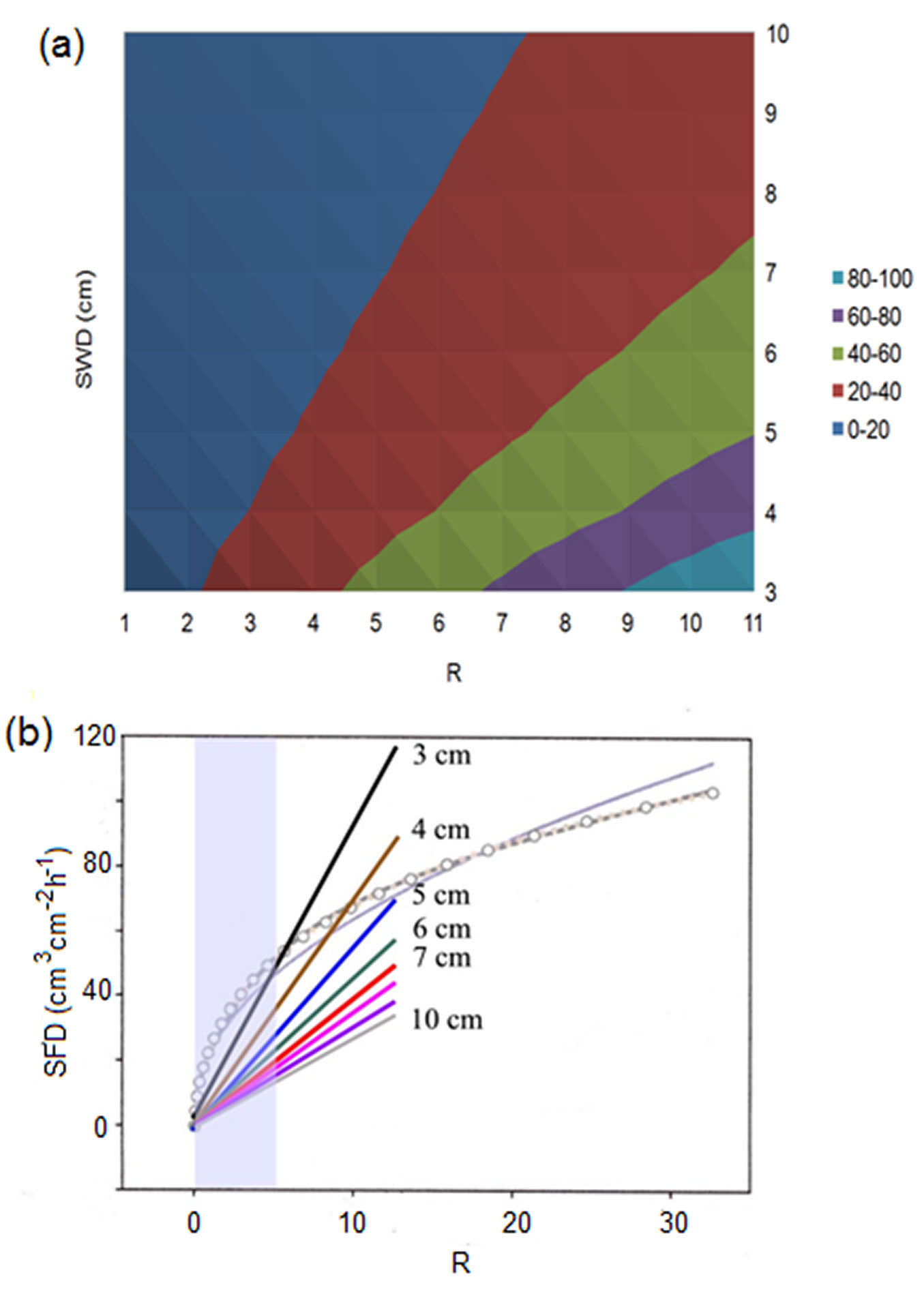
As L_sw widely varies between different trees, species and even within the same tree, this leads to a range of calculated q_s under the same R when calculations for different L_sw are made with the original equation (see Fig. 4b). Very similar results were reported recently by Fuchs et al. ([11]) when they plotted the gravimetrically determined sap flux density against HFD ratio (see Fig. 4 in [11]). We can see that the whole dataset have been divided in two well separated groups where the same values of R corresponded to higher sap flux densities for species with shorter L_sw (Fagus sylvatica) and to lower sap flux densities for deep sapwood species as Tilia and Acer (see Fig. S4 in [11] for visualization of the conductive sapwood area for these investigated diffuse-porous species). Several values of the HFD ratio larger than 7 (see Fig. 4 in [11]) were evidently in zone non-measurable by the HFD, due to dT_as approaching zero line. Including these values may lead to non-linear relationship between observed and predicted sap flux density found by these authors. The high variation among species (which is visible in the plot of gravimetric sap flux density vs. HFD ratio) disappeared when the comparison was done between sap flux densities (observed and predicted according to the original equation by [28], [30]), where the influence of L_sw was taken into account by including it as divisor in eqn. 4 (compare Fig. 4 and Fig. 1 in the above-mentioned paper). Thus, these authors directly confirmed the HFD principle, finding a certain dependence of sap flux density calculation relative to L_sw. The between-stem variation of sap flux density still observed by Fuchs et al. ([11]) for all investigated species (see Fig. 1) was evidently connected with the use of only one HFD sensor per stem, although it was shown that circumferential variability of sap flux density exists even in cut stem segments ([38], [11]).

Conversely, Vandegehuchte & Steppe ([45]) suggested the mathematical equation relating sap flux density with R independently from L_sw. When we compare the relationship between R and sap flux densities calculated for trees with different sapwood depths (according the original eqn. 4) with the 2D mathematical relation between modelled sap flux density and R suggested by Vandegehuchte & Steppe ([45], where this relationship is shown for certain wood properties in Fig. 7) we notice a large discrepancy in results (Fig. 4b). According to the equation suggested by the above authors, all earlier published HFD results should largely underestimate q_s especially for low fluxes and deeper sapwood (up to 400% or even more). This was not supported, however, even by their own data ([38]).

A simplified equation for scaling-up flow rate measurements to the tree level

To scale up sap flow to the tree level, sapwood area and radial variability of SFD should be known. Application of multi-point HFD sensors allows not only accurate measures of the sap flow radial profile ([39], [11]) but also correct estimates of the thickness of conducting sapwood from these measures ([2], [3]). To avoid difficulties related to the use of L_sw during the scaling procedure for trees with L_sw deeper than it could be estimated from sap flow radial profile, a simplified approach was recently proposed ([25]). By applying simple mathematical procedures, it was shown that sap flow per tree can be calculated as the average of SFS_i multiplied by the circumference a_i where the i-thermocouple of the sensor is situated. In the case of known sapwood depth (reachable by a sensor), results of flow up-scaling are identical after using both the simplified and the original approach, where the total sap flow is the product of summing up sap flow in individual annuli, which is calculated by multiplying sap flux density at a particular radial depth by the corresponding area of the annulus. This also indirectly confirms the accuracy of using L_sw in the original eqn. 4. It is interesting to point out that the simplified approach, surprisingly, leads to a scaling-up procedure similar to that used in the THB method ([7]). The only difference is that to scale up sap flow to the tree level, SFS of the THB (measured in the certain depths of sapwood) is multiplied by the circumference of the stem xylem radius at the height of measurements, whereas in the HFD, the total sap flow is the average of all measured SFS_i multiplied by the circumference a_i at each thermocouple position. Thus, in contrast with stable scaled-up sap flow using the HFD, results would be depended on thermometer placement along xylem radius for the THB.

  K value 

What is K-value and how is it measured?

As we have shown, K-value is an extremely important parameter characterizing the conducting properties at the sensor insertion place under local, specific measurement conditions. It involves information about the basic wood properties and heat conductivity in both axial and tangential directions in a tangential section of a tree organ. K-value depends on the sensor geometry (the distances of thermocouples from the heater) and the surrounding conditions, including power supply levels and the degree of insulation. It also depends on the length of the heater and its relative position in the SW/HW.

K-values are usually in the range of 1-4 °C for different species and situations in the case of sufficient but not excessive heating. K-value can be stable or may vary substantially along the radius and/or circumference, even in the same tree. It is common for higher values of K (for example, in the inner sapwood) to correspond to lower values of R, given that the real temperature of a heater is not homogeneous, and at the SW/HW border (where sap flow is low) the heater temperature may be largely influenced by close heat storage in HW. This is not always the case, as K-value represents the integral of several mutually supportive or antagonistic factors. Radial and circumferential variations of K-value may be used, for example, as an indicator of sapwood asymmetry or as evidence of decay in HW, etc.

K-values typically increase with sapwood depth in trees with deep sapwood (in conifer or diffuse-porous wood types). This is not, however, strictly always the case. For example, in one Douglas-fir tree measured from different sides, several radial variations of K were found; on one side, the typical radial trend for conifers was observed, while K-values on the other two sides either did not change substantially along the measured xylem radius or they decreased moving toward the inner xylem. This could be caused by an internal variation of wood structure (for example, the absence or presence of rot). On the other hand, the relative proportional length of the heater in SW/HW, or flow rates in the outer and inner xylem, may also play a certain role. The example of sap flow measurements in seven spruce trees is shown in Fig. S6 (Supplementary material). In three trees where flow rates in the outer xylem were very high, K-values were lower as compared to the inner xylem and to the other four trees recording lower R. In these four trees with comparable low flow rates along xylem radius, radial trends between K and R were rather similar, with no large differences between xylem layers. Radial variations of K-values which either remained unchanged or declined with increasing sapwood depth were observed quite regularly in trees with shallow sapwood depth such as oak, olive or eucalyptus. Interestingly, these trees are all hardwood species.

K-values can be determined even without zero flow conditions via linear extrapolation of the left upper part of the curve of dT_as corresponding to lower R up to intersecting Y axis. This removes the need to create zero flow conditions to determine the K-value, representing an additional advantage of the HFD method. To demonstrate this, I conducted two gradual cuttings of all shoots of a big branch of Tilia cordata tree on which a multi-point HFD sensor was installed. This resulted in zero flow in the branch, thus confirming the correctness of the linear extrapolation made before both cuttings in K-diagrams in order to determine K-values (see Fig. 7 in [34] where example for one xylem depth is presented). A larger scale for R represented in a K-diagram will produce more accurate K-values. For this reason, flow measurements taken on a time scale of no less than one day should be used to create a K-diagram. Sap flow measurements conducted during dry periods when high night values of R are more likely, can make it more difficult to determine accurate K-values. In such cases, either flow measurements should be taken over a longer period (to include rain or fog events, which decrease transpiration and sap flow) or for shorter time intervals a separate experiment should be conducted using cuttings, foliage spraying or localized irrigation applied from the tree side which is the opposite to that one where sap flow measurements are carried out. Localized irrigation during drought creates the conditions for horizontal hydraulic redistribution from irrigated to non-irrigated tree sides and by consequence, for negative sap flow (or at least decreased flow) in the non-irrigated side ([32]). This is a fast, non-destructive and effective treatment for increasing the scale of R. An example is shown in Fig. S7 (Supplementary material) which illustrates an accurate determination of K-value during drought with help of such treatment, when Douglas-fir tree was locally irrigated from the side opposite to sap flow recording.

Is K-value stable or varied, and for how long?

Although external impacts can be compensated by K-values, special care is recommended to maintain measurement conditions. When the object being measured is well protected from any external changes through sufficient insulation and power supply is well regulated, data processing is easier as K-values typically remain constant over very long periods, up to several seasons, as it occurred for example in a large deep root of Quercus suber under constant conditions of excess underground water (Fig. S8a, Supplementary material). If K-values do change even when external influences are minimized, it is possible to interpret the data by considering intrinsic transformations that, for example, occur when trees are subjected to severe drought and gradual tissue desiccation, as it was observed in the example of deep xylem layers of a spruce tree (Fig. S8b). Under such conditions, it is important to correct calculations by changeable K-values (Fig. S9, Supplementary material). Records of dT_as may help to select appropriate time intervals (weeks or days) for the new K-value determination: in the case shown in Fig. S9 the new K-values were determined when night maxima of dT_as started to shift to higher values. Abrupt changes of K-value are usually connected with sudden changes in surrounding conditions. Examples of objective correction of measurements by changeable K-value are presented in the next two sections.

Influence of insulation

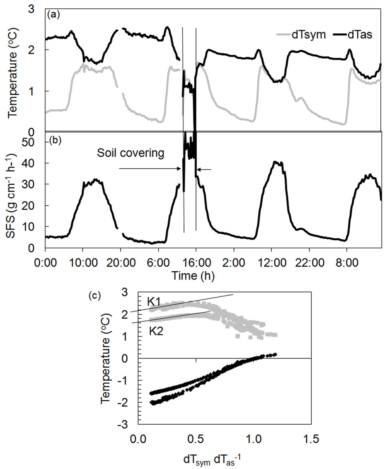
Fig. 5 shows an example of how rapid changes in local conditions can sharply influence measurements. A root of a Quercus ilex tree was partially opened for sensor installation. After three days, this root together with the sensor was covered again by a layer of soil. Although covering influenced the temperature differences recorded (Fig. 5a), calculated sap flow did not change (Fig. 5b) in response to corrected K-values (Fig. 5c). Such corrections can be made at any time and will not affect the collected dataset. Similar compensation also can be applied, for example, in the event of an abrupt change in power supply.

Fig. 5 - Dynamics of temperature gradients (a), sap flow per section (b) and K-diagram (c) for a root of a Quercus ilex tree. Vertical lines denote changes of surrounding conditions around the root (it was covered by soil after being open several days due to sensors installation). Clear separation of data on two sets depending on different surrounding conditions (open or covered by soil) is well visible in the K-diagram with different K-values for each dataset: K1 - before and K2 - after soil covering.

  Enlarge/Shrink   Download   Full Width  Open in Viewer

Sap flow measurements with or without sleeves

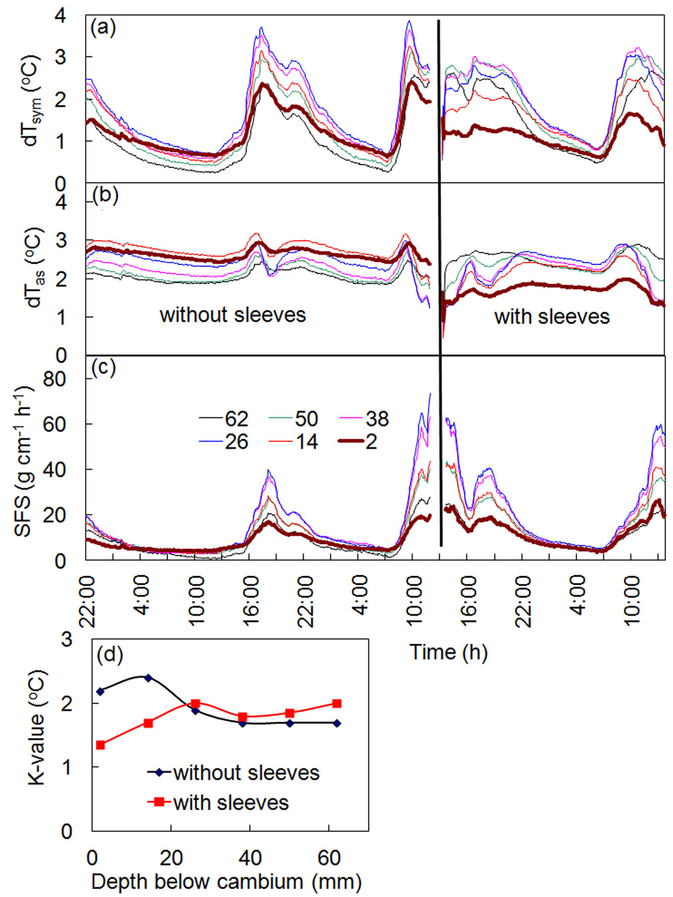
Initially, long multi-point HFD sensors inserted deeply into a stem xylem required a special tool for dismantling. In the case of long-term measurements, particularly in conifers, it became evident that removing the sensors, even with the help of this tool, was virtually impossible. It was very common for needles inserted into xylem to be broken during dismantling. Considering the unique ability of the HFD method to compensate for any changes to localized measurement conditions through K-value, it was suggested the use of stainless sleeves inserted into holes in the stem xylem before sensor installation. Sensor needles could then be inserted into the sleeves, with the additional advantage of avoiding any direct contact between the needle and the xylem. Experiments conducted on several species using this approach confirmed that this was the correct solution. The results of an experiment carried out on a spruce tree using the above procedure are shown in Fig. 6. The HFD sensor was first installed in a spruce stem directly into drilled holes 1.6 mm in diameter, and sap flow measurements were conducted over 2 days. Shortly following, at midday in full sun, the sensor was dismantled and the holes were enlarged up to 2.1 mm in diameter. Sleeves with outer diameters of 2 mm were then inserted into these same holes. The distal end of each sleeve was closed in order to prevent resin from entering. The inner diameter of sleeves was 1.6 mm where the needles of the sensor (with an outer diameter of 1.5 mm) were easily installed. Fig. 6a and Fig. 6b show that the process of sleeve insertion clearly changed the temperature differences recorded at the place of measurements. However, K-values in all measured depths also changed (Fig. 6d), effectively compensating for differences in recorded temperatures caused by the sleeves. The final result is that the calculated sap flow and the shape of sap flow radial profiles remain as they were before sleeves insertion (Fig. 6c).

Fig. 6 - Records of temperature differences dT_sym (a) and dT_as (b), sap flow per section, SFS (c), and K-values (d) for a spruce tree before and after sleeves insertion. Numbers in the legend indicate the depth of sapwood (in mm) where measurements were conducted. The time of sleeve insertion is marked by a thick vertical line.

  Enlarge/Shrink   Download   Full Width  Open in Viewer

Abrupt changes in sap flow do not influence K-value

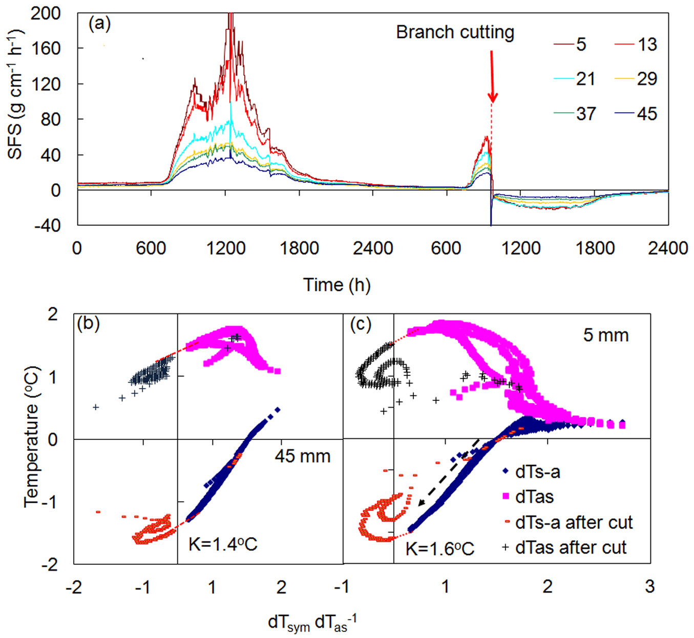
An interesting feature of the K-diagram is that it makes it possible to distinguish between reasons driving changes in temperature gradients recorded around a linear heater, or specifically, to determine if those alterations occurred as a result of conduction or convection. The above examples (Fig. 5, Fig. 6) illustrate the case of temperature differences modified by sudden external changes to heat conduction at the measurement place. In both cases, these changes were reflected in altered K-values, whereas sap flow rates (or R) were not altered. Fig. 7a demonstrates the opposite case, when an abrupt decrease in sap flow occurring throughout the whole sapwood was recorded in a stem of a Quercus suber tree, as a consequence of the abrupt cutting of a large branch above the multi-point HFD sensor ([9]). K-diagrams for two xylem depths (Fig. 7b, Fig. 7c) clearly indicate a sharp decrease of R up to negative values (due to abrupt changes in water potential gradients after replacement of negative water potential in the crown via positive atmospheric pressure localized to the cut branch above the sensor). Curves of temperature differences, interrupted by the cutting, passed Y axis in the same place showing the same K-value, as no changes to heat conduction had occurred at the place of sap flow measurement (situated several meters below the cut).

Fig. 7 - Sap flow dynamics in stem of a Quercus suber tree (a) and K-diagrams for the shallow (b) and deep (c) layers of sapwood. Sap flow was measured at six xylem depths below cambium (shown in legend, mm). Red arrow (a) indicate the time of cutting of a large branch. Black dashed arrow (c) indicates drop of sap flow in stem due to cutting the branch above the sensor. K-values showed no changes, as they were determined using the line connecting temperature curves before and after cut (data shown with permission of Teresa David).

  Enlarge/Shrink   Download   Full Width  Open in Viewer

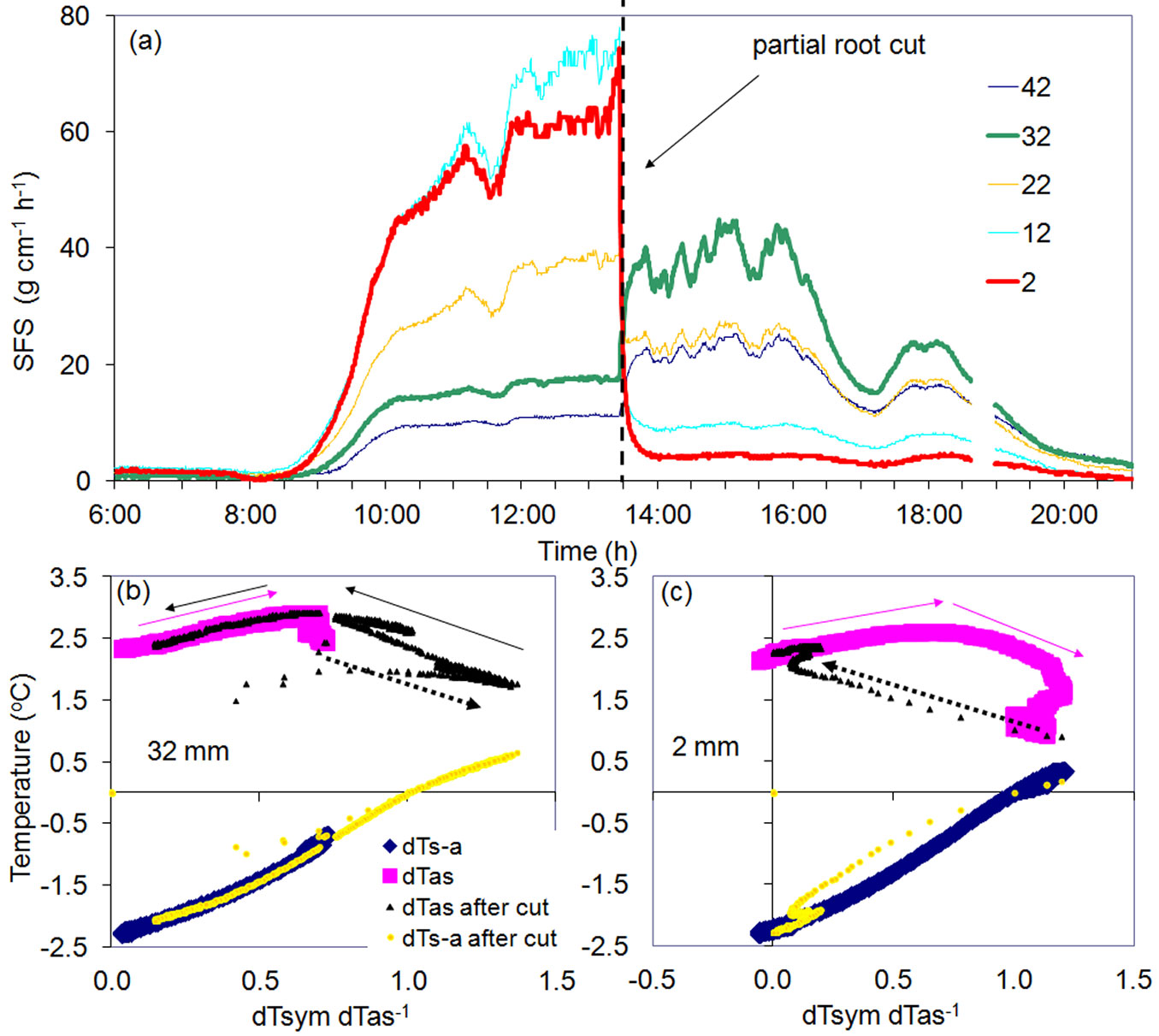
Another remarkable example was observed during the partial cutting of a large root of a Quercus petrea tree up to a depth of 23 mm below the cambium and 5 cm below the point where the multi-point sensor was installed in that root. The sensor was configured with thermocouples 10 mm apart with the first one positioned at a depth of 2 mm below the cambium. Flows immediately decreased in all the three outer layers corresponding to the depth of the cut (Fig. 8a). Flow increased, however, at the same time in the two inner undamaged xylem layers. Dramatic changes in temperatures resulting from the partial root cut were reflected in all K-diagrams: two are shown for the inner (Fig. 8b) and the outer (Fig. 8c) xylem. Both K-diagrams maintained the same shape and the same K-value. In both cases, all changes occurred due only to modified flow rates reflected in R changes. R increased in the inner xylem to a level which was never has been observed before the partial cutting. Following the cutting, flow in the undamaged xylem layer doubled as compared to the normal level. New temperature differences (not recorded before cutting) supported the same K-diagram type for its upper level which was not reached before cutting (R abruptly increased up to 1.4), then R gradually decreased the next night following the same curve previously recorded. These new daily R fluctuations were observed to repeat over the next days. This is an excellent example of how the reserve capacities of root xylem may facilitate or support water conductance when necessary. The opposite was observed in the outer xylem. The ratio R abruptly decreased from its midday maximum (R around 1.2) descending to almost zero, while again, maintaining the same daily curve with the same K-value. Using K-diagrams makes it easy to calculate transition periods from one stable flow level to the next, notably because each point represents 30 seconds in the presented case. This transition period was around 10 minutes for the inner xylem, and roughly 15 minutes for the outer xylem. Even abrupt R changes had the opposite character; there were no changes in K-value for either case because conductance conditions (wood type, power supply, isolation, etc.) remained constant.

Fig. 8 - Daily dynamics of sap flow in root xylem of a Quercus petrea tree at different depths below cambium (a) and K-diagrams for the inner (b) and the outer (c) root xylem. Sap flow was measured with 30 sec interval at five depths below cambium (shown in legend, mm). In the middle of a bright day the root was partially cut (dashed vertical line in a) to the depth of 23 mm. Pink arrows in (b) and (c) indicate routine increase of R from the morning until midday before the cutting occurred. Black dashed arrows indicate fast transition period of flow increase (b) or decrease (c) due to partial root cut. Full black arrows in (b) show the decrease of R from midday until night following the cutting.

  Enlarge/Shrink   Download   Full Width  Open in Viewer

The above examples (Fig. 5 to Fig. 8) clearly demonstrate that both processes (conduction and convection, which are mutually interconnected in a real tree) are well reflected by K-values (changes of conduction conditions, recorded along the Y axis) and/or R values (changes caused by convection, recorded along the X axis) through the use of K-diagrams.

  Types of K-diagrams 

There are basically two main types of K-diagrams (Fig. 9). Type 1 can be considered as “classical”, as it occurs when temperature courses form a daily loop, with the dT_sym/dT_as ratio gradually increasing from the morning to the afternoon and then decreasing until nightfall (Fig. 9a). Type 2 is responsible for the so-called “McDonalds effect”, with the dT_sym/dT_as ratio gradually increasing in the morning, suddenly “turns back” at midday, then increasing again in the afternoon before finally decreasing at night (Fig. 9b). The difference between the two types of K-diagrams relates directly to the different mutual position of dT_sym and dT_as under higher flow rate conditions. When flow rates are low, dT_as is always higher than dT_sym. Once both temperature gradients are equalized (easily characterized by dT_s-a as equal to zero and when dT_sym/dT_as ratio equals to 1), dT_as could be either lower than dT_sym (type 1) or higher (type 2).

Fig. 9 - Different types of K-diagram constructed for a lime (a) and oak (b) trees and K/R-diagram (c) made for the same dataset presented in (b). K is equal to 3 °C in both examples.

  Enlarge/Shrink   Download   Full Width  Open in Viewer

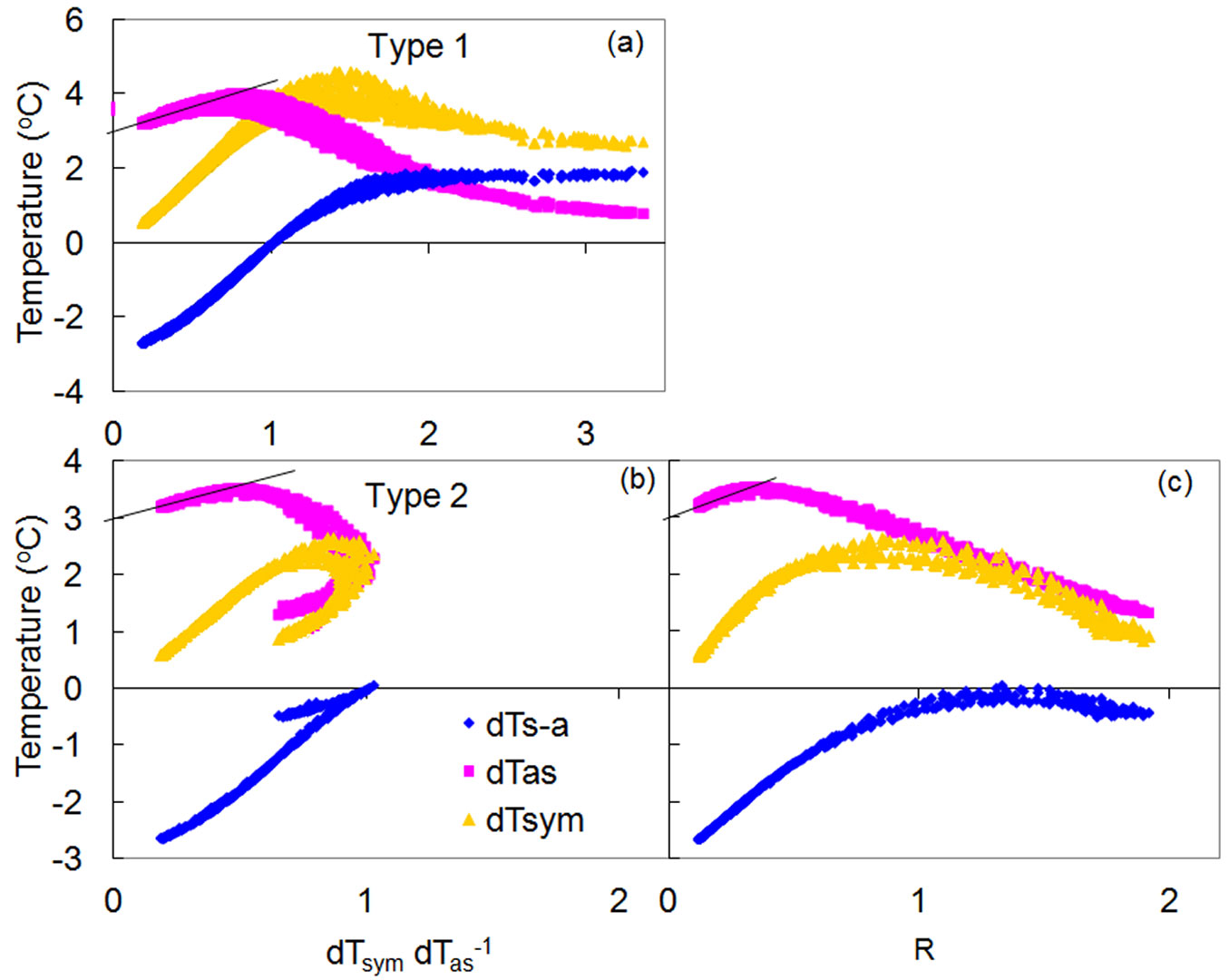
Both types of K-diagrams can be detected within a single species and among different species, and even within the same tree, in its different organs or stem sides, or at different depths of stem xylem. Several types of K-diagrams can even occur at the same measuring point during long-term monitoring periods. In Fig. S10 (Supplementary material) the K-diagram recorded in the stem of a spruce tree subjected to increasing drought conditions gradually changed from type 1 to type 2.

  K/R-diagram 

Use of temperature difference (K+dT_s-a) instead of dT_sym helps to overcome the negative “McDonalds effect” during sap flow calculation. We can see this when the alternate ratio between temperature differences, R, is used for flux analysis (Fig. 9c). The relationship between R and temperature differences dT_as and dT_s-a is called a K/R-diagram. K/R-diagrams differ from K-diagrams (type 1) by magnitude of the ratio (K+dT_s-a)/dT_as which is approximately twice as large then the dT_sym/dT_as ratio (this does not fit for the type 2 of K-diagram). This difference, however, is compensated in the final formula for sap flow calculation by distances that are twice the distance between thermocouples for dT_sym than the axial distance Z_ax between thermocouples for dT_s-a (Z_sym=2 Z_ax).

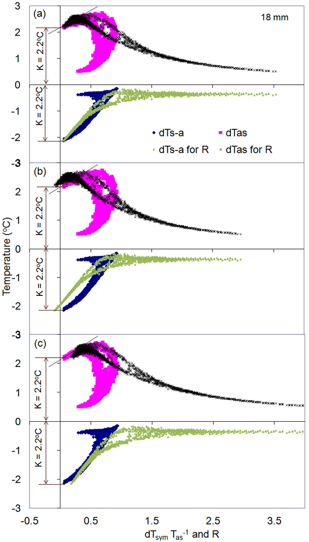
K/R-diagrams are particularly useful for checking the accuracy of K-values obtained, which is important in the case without zero-flow conditions or for more complicate types of K-diagrams. To do that, it is helpful to present both diagrams together in one graph: a K-diagram for resolving K-values and a K/R-diagram for checking the correctness of the determined K-values (Fig. 10). In the case of correct K-values, both diagrams will indicate the same magnitude for K-value (Fig. 10a). In the case of incorrect K-values, the K/R-diagram deviates from a K-diagram and from equality between dT_as and dT_s-a for zero flow conditions (Fig. 10b, Fig. 10c). The figure clearly shows that the accuracy in calculating sap flux density greatly depends on a correct determination of K-values. Errors in K-values may result in underestimation (Fig. 10b) or overestimation (Fig. 10c) of SFS (Fig. 10a). As such, accurate whole-tree sap flow rates are also highly dependent on a correct determination of K-values.

Fig. 10 - K-diagram and K/R-diagram presented together for two months of sap flow measurements in the stem of a Q. suber tree at xylem depth 18 mm below cambium. (a) K-value was determined correctly (K-value is identical in both diagrams) or wrong (match in K-value for both b and c diagrams is lost). Note the independence of K-diagram from correctness of K-value determination, whereas incorrect K-value clear violates the equality between dT_as and dT_s-a on K/R-diagrams: decrease of K-value from its correct magnitude leads to higher dT_as and lower dT_s-a (in absolute value) when these temperature differences cross Y-axis (b). The opposite occurs when K-value will be taken higher than its correct magnitude (c). Correspondent to wrong K-value, also R will be wrong: underestimated in (b) or overestimated in (c) compared with the correct value in (a).

  Enlarge/Shrink   Download   Full Width  Open in Viewer

To summarize, K-diagrams are important for the following reasons:

• for determining K values;
• for checking the correctness of installation (parallelism of long needles): dT_as should be equal to dT_s-a under zero flow;
• for understanding what causes changes in the recorded temperatures: conduction or convection;
• for showing radial changes of dT;
• K/R-diagrams help to assess the accuracy of K values;
• K/R-diagrams have to capacity to transform from type 2 of K diagram into type 1, avoiding the negative “McDonalds” effect during sap flow calculation.

  Acknowledgments 

The author wishes to thank Jan Cermák for building the first multi-point HFD sensors and Valerij Nadezhdin for the overall technical support.

  References

  Supplementary Material

Fig. S1 - Cross-sections and photos of stems of a Tilia cordata tree with infra-red images of the heat field around a linear heater.
Fig. S2 - Tangential and radial IR images of a heat field in stem of a Tilia cordata tree with schemes of sensor displacement.
Fig. S3 - Dynamics of symmetrical temperature difference, dT_sym, and sap flux density in a lateral root of a Quercus suber tree, measured at the end of dry and the beginning of wet periods.
Fig. S4 - Dynamics of dT_as and SFS in pear tree before and after corrections of K-values, altered due to changes in the length of the heater in a stem, as a result of moving the heater out at 1 cm.
Fig. S5 - Sap flow dynamics measured by the same multi-point HFD sensor in the stem of a Quercus suber tree from four different stem sides.
Fig. S6 - Dependences of R and K-values from depth of measurement in sapwood of seven spruce trees.
Fig. S7 - K-diagrams constructed for a Douglas-fir tree before and after application of localized irrigation.
Fig. S8 - K/R-diagrams for a Quercus suber large sinker root and spruce stem measured during 7 months at xylem depth of 3 cm from the cambium.
Fig. S9 - Sap flow dynamics measured in stem of a spruce tree in two xylem depths calculated with and without correction of K-value.
Fig. S10 - Dynamics of temperature differences, sap flow and K-diagram for a spruce tree measured in a dry period.