A comparative study of four approaches to assess phenology of Populus in a short-rotation coppice culture
iForest - Biogeosciences and Forestry, Volume 9, Issue 5, Pages 682-689 (2016)
doi: https://doi.org/10.3832/ifor1800-009
Published: May 12, 2016 - Copyright © 2016 SISEF
Research Articles
Abstract
We compared four approaches to assess phenology in a short-rotation coppice culture with 12 poplar (Populus) genotypes. The four approaches quantified phenology at different spatial scales and with different temporal resolutions: (i) visual observations of bud phenology; (ii) measurements of leaf area index; (iii) webcam images; and (iv) satellite images. For validation purposes we applied the four approaches during two years: the year preceding a coppice event and the year following the coppice event. The delayed spring greenup and the faster canopy development in the year after coppicing (as compared to the year before coppicing) were similarly quantified by the four approaches. The four approaches detected very similar seasonal changes in phenology, although they had different spatial scales and a different temporal resolution. The onset of autumn senescence after coppicing remained the same as in the year before coppicing according to the bud set observations, but it started earlier according to the webcam images, and later according to the MODIS images. In comparison to the year before coppicing, the growing season - in terms of leaf area duration - was shorter in the year after coppicing, while the leaf area index was higher.
Keywords
Introduction
Phenology is defined as the study of the timing of recurrent biological events, e.g., alternating periods of active growth and dormancy in deciduous trees in temperate regions ([38]). These recurrent biological events are controlled by genetic ([29]) and environmental factors ([10], [16], [43]), as well as by community structure and competition ([38]). Phenology is used as an integrative measure of plant responses to environmental changes ([38], [44]). The timings of bud burst and bud set are adapted to the local climate ([17], [56]); they are crucial for tree growth ([45]), survival ([23], [30], [31]), and reproduction ([5], [26]). Within the Populus genus there is a large genotypic variation in, and a strong genetic control of the timing of bud burst ([14], [32]) and of bud set ([39], [40]). In (intensively) managed forest ecosystems (e.g., short-rotation coppices - SRCs) additional management factors also alter the pattern of annual phenological events. SRCs are often established with Populus species and coppicing is the most influential, recurrent management factor, whereby all above-ground biomass is harvested ([18]). However, data on the impact of coppicing on phenology are largely missing ([33]).
Plant phenology is quantified via different approaches at different spatial scales and with different temporal resolutions. Visual field observations of single species are the oldest and the most direct approach ([41], [49]). Monitoring the leaf area index (LAI) of experimental areas of limited size is also used to quantify phenology ([1], [11], [36]). More recently, flux measurements ([27], [46]) and digital repeated photography ([37], [35], [20], [24], [25]) have automated phenological observations and increased the spatial scale of observation. The use of satellite images represents the most recent advanced approach in phenological studies, extending the spatial ([21]) and temporal ([28], [12], [57]) scales to continents and decades, respectively. Only a few studies have compared different methods to monitor the phenology of forest ecosystems ([13], [25]), though this is of particular interest for the validation of satellite images ([47]). At present we lack such methodological comparisons for intensively managed ecosystems as SRCs. The specific nature of SRCs at the interface between agriculture and forestry also allows testing of new indices used for monitoring phenology. The wide dynamic range vegetation index (WDRVI) for example, which is a satellite based MODIS vegetation index, has been applied for agricultural purposes, but has not yet been thoroughly tested for forest plantations ([22]).
In this study we compared different methods to monitor phenology. We applied four approaches at an operational SRC over two distinct years, i.e., the year before and the year after coppicing. The four approaches were: (i) visual observations of bud phenology; (ii) measurements of LAI; (iii) webcam images; and (iv) satellite images. The primary objective of this study was to compare the four approaches to the phenological changes and among each other.
Materials and methods
Site description
All observations were made at the operational SRC plantation “POPFULL” in Lochristi, Belgium (51° 06′ N, 3° 51′ E - ⇒ http:// uahost.uantwerpen.be/popfull). The plantation was established on 7-10 April 2010 ([8]) and consisted of 12 different poplar (Populus) genotypes planted in mono-genotypic blocks, on former agricultural and pasture land ([53]). A tree density of 8000 plants ha-1 was achieved with a double-row planting scheme: hardwood cuttings were planted 1.1 m apart with alternating inter-row distances of 0.75 and 1.50 m. The entire plantation was harvested for the first time after two years of growth on 2-3 February 2012, i.e., on day of year (DOY) 33-34 ([3]). The present study focuses on the year before (2011, i.e., the second year of the first rotation) and the year after the harvest (2012, i.e., first year of the second rotation). Before coppicing the majority of trees had one single stem, while after coppicing the plantation consisted of coppiced stools with up to 46 shoots per stool ([52]).
A meteorological mast in the plantation continuously monitored all meteorological variables from May 2010 onward. Photosynthetically active radiation (PAR, 400-700 nm) was continuously recorded above the canopy using a quantum sensor (LI-190, LiCor Inc., USA - [59]). Volumetric soil water content was measured horizontally at specific depths of 1 m, 60 cm, 40 cm, 30 cm, and 20 cm below the surface, using soil moisture probes (TDR model CS616, Campbell Scientific, USA). Air temperature was recorded using a Vaisala probe (model HMP45C, Vaisala, Finland) mounted on a telescopic mast next to the meteorological mast. For a complete description of all instruments and sensors on the meteorological mast, the reader is referred to an earlier publication ([59]).
Assessments of phenology
Visual observations of bud phenology
Bud burst and bud set were visually and intensively scored per genotype during the spring and the autumn, before (year 2011) and after (year 2012) coppicing. We applied the bud burst scoring system (with five discrete classes) previously developed and validated for poplar ([33], [51] - Fig. 1). During the spring of 2011 (late February - mid-May) the gradual process of bud burst and leaf development was quantified each week by assigning scores to eight plots of four trees per genotype. Bud burst scores were averaged per DOY. In the spring of 2012 (early April - mid-May) one of the five scores was assigned to each monogenotypic block as a whole on a weekly basis. In 2011 observations were made on the buds of the upper part of the main current-year axis, while in 2012 observations were made on the buds of the stumps.
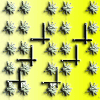
Fig. 1 - Schematic presentation of the five discrete classes used for scoring bud burst in poplar. (1) Dormant bud completely encapsulated by the bud scales, completely dry outlook and brown color; (2) buds sprouting, with a tip of the small leaves emerging out of the scales, leaves cannot be observed individually; (3) buds completely opened with leaves still clustered together, scales still present, leaves individually visible but folded on it; (4): leaves diverging with their blades still rolled up, scales may be present or absent, folded leaves starting to open, leaf venation visible; (5): leaves completely unfolded (but smaller in size than mature ones), lengthening of the axis of the shoot evident, scales absent, development of leaves from the elongation of the lateral branch ([33], [51]).
Autumn phenology, i.e., the end of tree height growth and of leaf production, was assessed using a bud set scoring system (with seven discrete classes) established and validated for poplar ([40] - Fig. 2). Analogously to bud burst, scores were assigned each week to eight plots of four trees of each genotype in the autumn of 2011 (late August - early October). In the autumn of 2012 (late August - mid-October) two plots of four trees were assigned to one of the seven classes on a weekly basis and these values were averaged per DOY. As for the bud burst scoring, we scored the apical bud on the main current-year axis in 2011 and the apical buds on all resprouting axes in 2012.
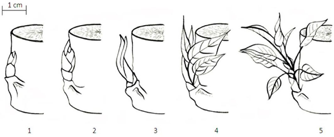
Fig. 2 - Schematic presentation of the seven discrete classes used for scoring bud set in poplar. (0): Apical bud red-brown; (0.5): apical bud fully closed, color between green and red, stipules of the two last leaves still green; (1): apical bud not fully closed, bud scales predominantly green, no more rolled-up leaves; (1.5): transition from shoot to bud structure, color of second last leaf is comparable to older leaves, last leaf partially rolled; (2): shoot/internode growth reduced, second last leaf fully stretched, last leaf bright green; (2.5): last leaves still rolled-up, last leaves at equal height, internodes become shorter; (3): apical shoot fully growing, > 2 rolled-up young leaves ([51], [33]).
Leaf area index measurements
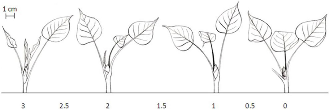
Leaf area index (LAI) was indirectly measured using the LI-2200 plant canopy analyser (LiCor Inc., USA) with a 45° view cap. The measurements were taken on a regular basis (± every two weeks) during the year before and the year after coppicing in 96 predetermined plots equally spread over the different genotypes and the two former land use types: 12 genotypes × 2 former land uses × 4 replicates. Per plot, two diagonal transects were made between the planted rows (Fig. 3). Per transect, six sample measurements were taken: three parallel to the rows and three perpendicular to the rows ([7] - Fig. 3). Using the software FV2200 (version 1.0.0, LiCor Inc., USA), sample measurements were combined to generate one LAI value per plot, which was averaged to one value for the entire plantation. In the year after coppicing, the onset of spring greenup could not be monitored because leaves were too close to the ground, hence inhibiting correct below-canopy light measurements.
Fig. 3 - Schematic representation of one plot used for leaf area index (LAI) measurements in the double-row planting design. Green silhouettes indicate individual coppiced stumps; dotted lines indicate the direction of the row. Thick black bars represent the LI-2200 LAI instrument, with the white tip as the actual light sensor.
Webcam image acquisition
Webcam images were obtained using a standard commercially available webcam (AXIS P1344, Axis Communications AB, Sweden) mounted in a weatherproof enclosure; full technical specifications are available online ([2]). The webcam was installed on the telescopic mast at a height of 4 m, facing west-southwest and set at an angle of 20° below horizontal ([20]). The webcam remained in the same position and orientation during the two years of this study. Images were stored as minimally compressed JPEG files (1024 × 768 pixels). Analyses were performed on a rectangular region of interest (ROI - Fig. 4). Images were collected every day at 10:00 AM (solar time). Images with raindrops or direct sunlight on the lens were discarded, keeping 323 (out of 365) images for 2011 and 331 (out of 366) images for 2012.
Fig. 4 - Example of webcam image (date: Sep 22, 2012) in the year after coppicing of the poplar short-rotation coppice (SRC). The region of interest (ROI) used for the analyses is indicated by the black rectangle.
The phenocam Matlab script (available at ⇒ http://phenocam.sr.unh.edu/webcam/) was used to analyse the digital image files ([37]). Webcam color channel information (i.e., digital numbers - DNs) was extracted from the JPEG files and averaged across the ROI for red, green and blue (RGB) color channel and expressed in percentage. The overall brightness of the ROI was calculated as the sum of the DN of the three color channels (eqn. 1):
The relative channel brightness of each channel (i.e., channel %) was calculated by dividing the channel DN by the total RGB DN ([37] - eqn. 2):
For the ROI of each image the excess green index (ExG) was calculated as the difference in divergence of both the red and the blue channels from the green channel % as described by Richardson et al. ([37]) - eqn. 3:
This index is commonly used to discriminate leaf cover from the soil background in forest canopy phenology studies ([20]).
Using the method described by Zhang et al. ([58]) and applied by Hufkens et al. ([20]), the DOY phenophase transition dates were estimated as follows: (i) ExGin, the date of spring onset; (ii) ExGmax, when maximum green leaf area was reached; (iii) ExGde, the date when photosynthetic activity and green leaf area began to rapidly decline; (iv) ExGmin, the date at which physiological activity became near to zero. To determine the transition dates, we used the ExG data spanning the period between DOY 50-150 (in 2011) and DOY 100-200 (in 2012) for the spring and between DOY 250-366 for the autumn. A single sigmoidal curve per season was fitted to the data in R ([34]), from which phenophase transition dates were extracted ([58] - eqn. 4 to eqn. 7):
Greenup (defined as ExGmax - ExGin) and senescence (defined as ExGmin - ExGde) duration were calculated to provide information about leaf development in spring and leaf shedding in autumn ([20]). Leaf area duration (LAD, calculated as ExGmin - ExGin) was determined as an indicator of the length of the growing season.
Satellite image processing (MODIS)
MODIS vegetation indices (NDVI and WDRVI) were calculated from MOD09GQ “MODIS/Terra Surface Reflectance Daily L2G Global 250m”. Each MOD09GQ pixel contained daily red and near-infrared reflectance data at a 250 m resolution as well as additional information on band quality, orbit and coverage, and number of observations. MODIS data were ordered and downloaded via the MODIS Adaptive Processing System (MODAPS) Services website. From this dataset, the following vegetation indices were calculated: (i) the normalized difference vegetation index (NDVI, [42] - eqn. 8):
and (ii) the wide dynamic range vegetation index (WDRVI, [15] - eqn. 9):
where ρred and ρNIR are reflectance values for respectively MODIS band 1 (620-670 nm) and band 2 (841-871 nm), and α is a weighing factor (i.e., 0.2 for row crops - [55]). MODIS data were resampled by using the Nearest Neighbour resampling algorithm and the selected projection was Geographic (i.e., GEO: WGS 84 lat/lon). From resampled and georeferenced MOD09GQ time-series for 2011 and 2012 we extracted one pixel (250 × 250 m) corresponding to the site coordinates for each day.
For the MODIS data quality check we used the available information retrieved in the MOD09GQ for band 1 (NIR) and band 2 (red). MOD09A1 pixel values represent the optimal reflectance values within a time window of 8-days. Only the pixels with the highest quality (e.g., clear sky conditions without snow) and flagged as “good” were selected and retained for further use. The MODIS data processing was compiled using the MATLAB software (MATLAB v. 2012a, MathWorks, Natick, MA, USA).
The method described by Zhang et al. ([58]) was used to derive the phenological transition dates from MODIS vegetation indices time series. The NDVI is the most widely used indicator related to vegetation greenness ([4]), while the WDRVI was recently developed as an expansion of the NDVI, to reduce the latter’s sensitivity to saturation effects ([54]).
Results
The growing seasons of 2011 and 2012 were very comparable in terms of climate conditions. The main meteorological variables - PAR (Fig. 5a) and air temperature (Fig. 5b) - were confined within comparable limits and showed similar patterns during both growing seasons. The volumetric soil water content (Fig. 5b) was in the same range for both growing seasons, although soils dried out more and earlier in the summer of 2011 as compared to 2012. This might be resulting from the larger amount of transpired water in 2011 as more above-ground biomass was present. The phenology assessed at bud and at plant level showed similar seasonal trends in 2011 and 2012. Bud burst (Fig. 5c) occurred at DOY 50-125 in the year before coppicing and lagged till DOY 75-150 in the year after coppicing. This lag time was the result of the coppicing in February 2012, as new buds had to be formed from meristematic cells on the coppiced stumps. Bud set, however, occurred in both years at DOY 225-275. In the year before coppicing the LAI (Fig. 5d) started to increase around the same time as the bud burst and the maximum seasonal LAI (2.4) was reached by the time bud set was completed. The direct effect of the coppice was evidenced by the LAI data, because these dropped from 0.33 (also known as the branch area index) to zero on DOY 33-34, the days on which the coppice was executed. The maximum seasonal LAI (5.7) was again reached by the time bud set was completed in the year after coppicing.
Fig. 5 - Environmental variables and phenological indicators measured at the short-rotation coppice plantation in the years 2011 (before coppicing) and 2012 (after coppicing). The coppice was carried out on 2-3 February 2012 (DOY 34-35) as indicated by the arrow at the bottom. (a) Photosynthetically active radiation (PAR, μmol m-2 s-1); (b) air temperature (°C) and volumetric soil water content (m3 m-3); (c) bud burst and bud set phenology expressed on a scale of discrete classes; (d) leaf area index (LAI, m2 m-2); (e) relative red, blue and green channel brightness (%, respectively in red, blue and green squares), and the excess green index (ExG, raw data and filtered data are shown) extracted from the webcam images; (f) normalized difference vegetation index (NDVI) and wide dynamic range vegetation index (WDRVI) from the MODIS satellite image.
The relative channel brightness derived from the webcam images (Fig. 5e) showed several clear phenological patterns. Taking into account the day-to-day variations, the red % decreased between DOY 75-125 (before coppicing) and DOY 100-150 (after coppicing); the autumn red signal was visible around DOY 325 in both years. Apart from minor day-to-day variations, the blue % remained fairly constant over both years. The green % had the least day-to-day variations, and showed a trend opposing the one observed for the red %. The green % dynamics were more expressed by the ExG (Fig. 5e). Spring greenup in the year before coppicing occurred in the last half of the period as quantified by the bud burst and LAI, while the leaf colours gradually changed between DOY 225 and 350 (Fig. 5e). Spring greenup took off after bud burst was completed in the year after coppicing, while the leaf colours changed as gradually as in the year before coppicing (Fig. 5e). The effect of coppicing is both directly and indirectly visible from our data. It is directly visible because the red, green and blue % converged to 33% (typical for snow cover on a bare soil) at the moment of the coppicing. In an indirect way, the coppice postponed the onset of spring greenup, thereby shortening the LAD by 63 days (as compared to the year before coppicing) and because the maximum seasonal ExG increased from 78 before coppicing to 93 after coppicing (Tab. 1). The maximum seasonal ExG values were reached earlier in the season in both years as compared to the maximum seasonal LAI values.
Tab. 1 - Dates of different phenological events derived from webcam (excess green index, ExG) and satellite (NDVI and WDRVI) images in the years before coppicing (2011) and after coppicing (2012). All dates are expressed in terms of day of year (DOY). (ExGin): onset of spring greenup; (ExGmax): start of maximum greenness, (ExGde): start of senescence; (ExGmin): start of minimum greenness; (NDVI): normalized difference vegetation index; (WDRVI): wide dynamic range vegetation index.
| Parameter | Webcam | NDVI | WDRVI | |||
|---|---|---|---|---|---|---|
| 2011 | 2012 | 2011 | 2012 | 2011 | 2012 | |
| ExGin | 65 | 121 | 64 | 104 | 80 | 148 |
| ExGmax | 131 | 178 | 184 | 200 | 200 | 200 |
| ExGde | 221 | 200 | 208 | 232 | 224 | 240 |
| ExGmin | 356 | 349 | 352 | 336 | 360 | 304 |
The NDVI and the WDRVI showed very comparable seasonal patterns in both years, although the growing season was more evident by the WDRVI in comparison to the NDVI (Fig. 5f). The NDVI confined the growing seasons within the same limits as shown by the webcam in the year before coppicing, while the WDRVI showed a lag phase of ≈20 days (Tab. 1). In the year after coppicing the webcam results reached their peak values ≈15 days later than the NDVI. The WDRVI quantified the growing season as starting later (≈25 days) and being shorter (≈70 days) than the growing season as quantified by the webcam. Both the NDVI and the WDRVI showed that the growing season started later (resp. 40 and 68 days) and ended earlier (resp. 16 and 64 days) in the year after coppicing as compared to the year before coppicing. Both MODIS vegetation indices were not accurate enough to identify the coppicing operation. The NDVI was more sensitive to small changes in phenology and hence responded more quickly to bud burst as compared to the WDRVI. On the other hand, bud set fell in the middle of the senescence period as estimated by both MODIS vegetation indices. The doubling of the maximum seasonal LAI value from the year before coppicing to the year after coppicing was neither translated in a doubling of the NDVI nor of the WDRVI; the NDVI and the WDRVI only slightly increased. The WDRVI was lower than the NDVI at LAI < 2, while the trend was the reverse at LAI > 2.
During senescence, the four approaches (visual observations of bud phenology, measurements of leaf area index, webcam images and satellite images) were triggered in a different way and thus also at a different time. The overall greenness obtained from both webcam and MODIS images slightly declined when older leaves got shaded by the younger leaves, because the percentage of sunlit leaves decreased relatively to the total amount of leaves. Over the entire growing season the number of young leaves relative to the total number of leaves declined, thereby causing a gradual decline in greenness. This was mainly visible in the ExG (Fig. 5c), as MODIS images (Fig. 5d) also incorporated understory weed species in the plantation. After the maximum seasonal LAI was reached, buds were set, but this bud set was not recognized in the webcam- and satellite-based phenological assessments.
Discussion
The four approaches (visual observations of bud phenology, measurements of leaf area index, webcam images and satellite images) to assess phenology clearly showed the seasonal patterns and yielded similar results, despite the methodological differences. For example, LAI values depend on light attenuation through the canopy, while the ExG, NDVI and WDRVI indices depend on canopy greenness. The four different approaches to assess phenology produced, however, different interpretations of phenology. During greenup all approaches were triggered at the same time, but in a different way: leaf buds opened, thereby unfolding leaves, which triggered the LAI by intercepting light; this also triggered the ExG because the young leaves are green. In turn this also triggered the two MODIS indices by introducing a different color palette to the observed area ([48], [36], [19], [25]).
The maximum seasonal LAI value in the year after coppicing was double the maximum seasonal LAI value in the year before coppicing. This could be explained by the transition from single- to multi-stem coppiced stools: up to 46 shoots per stool emerged after coppicing ([7], [52]). This increased amplitude in LAI in the year after coppicing was weakly represented by the ExG index, while it remained unnoticed by the NDVI and WDRVI indices. In general, the ExG and the NDVI indices saturate when the LAI surpasses 2.0 ([15]) or 2.5 ([24], [25]). Our results confirmed earlier findings on row crops ([15]) that showed that the NDVI predicted the start (ExGin) and the end (ExGmin) of the growing season (and thus, the LAD) better than the WDRVI. The WDRVI was better in representing amplitudinal differences in LAI at higher LAI values (i.e., the period of maximum greenness, from ExGmax until ExGde). Furthermore, the NDVI overestimates field observations ([9], [13]), but this could not be concluded from our data.
Ground validation (visual observations of bud phenology and measurements of leaf area index) of remote sensing data (webcam and satellite images) remains necessary and is still lacking for most vegetation types ([24], [58]). As evident from the present study, several critical considerations should be taken into account when comparing results from approaches at different spatial and temporal scales ([37], [35]). First, the steep rate of the spring greenup curve as observed by the webcam images might be exaggerated because of the oblique viewing angle of the webcam. This oblique viewing angle looks upon more layers of leaves as when it would face 90° downwards ([24]). The position and the angle of the webcam were chosen as a compromise to include as many trees in the field of view as possible and at the same time maximizing the resolution in the ROI during the growing season. Nevertheless, the field of view changed according to the cosine law: with increasing canopy height, the horizontal area visible by the webcam became smaller. Secondly, the extent of autumn senescence at the end of the growing season might be overestimated, as the ROI images integrated several different poplar genotypes, which differed in the timing of different phenological stages ([32], [6]). Therefore the webcam images aggregated the phenological responses of the different poplar genotypes, leading to an increased overall duration of spring greenup and autumn senescence ([20], [25]). However, the impact of coppicing on phenology was clearly visible. Thirdly, no white or grey reference panel was installed in the field of view of the webcam. The installation of a reference panel could lead to a more pronounced variability in the channel brightness due to changes in the quality and the quantity of incident solar radiation ([37], [27], [46]). Nevertheless, the timing of the different phenological events was clearly visible from our webcam images. Finally, the accuracy of the MODIS vegetation indices was limited to one pixel only, with considering geolocation details. Although this may not seem representative at first, the single pixel approach has been used before ([50]).
Conclusions
In conclusion, the four approaches to quantify phenological events agreed rather well and clearly reflected the effect of coppicing. Considering the different spatial scales and temporal resolutions of the four approaches, they all confirmed each other. However, it is important to keep the methodological differences and the different plant attributes assessed with every approach in mind when different approaches are compared or simultaneously applied.
Acknowledgements
This research has received funding from the European Research Council under the European Commission’s Seventh Framework Program (FP7/2007-2013) as ERC grant agreement n° 233366 (POPFULL). Further funding was provided by the Flemish government through the Hercules Foundation as Infrastructure Contract ZW09-06 and by the Methusalem Program. We gratefully acknowledge the technical support of Joris Cools and the logistic support of Kristof Mouton at the field site, as well as the useful suggestions by Koen Hufkens (Harvard University, USA).
References
Online | Gscholar
Gscholar
CrossRef | Gscholar
CrossRef | Gscholar
Gscholar
Gscholar
CrossRef | Gscholar
Online | Gscholar
Gscholar
CrossRef | Gscholar
CrossRef | Gscholar
CrossRef | Gscholar
Authors’ Info
Authors’ Affiliation
Jasper Bloemen
Manuela Balzarolo
Laura S Broeckx
Isabele Sarzi-Falchi
Melanie S Verlinden
Reinhart Ceulemans
University of Antwerp, Department of Biology, Research Center of Excellence on Plant and Vegetation Ecology, Universiteitsplein 1, B-2610 Wilrijk (Belgium)
University of Innsbruck, Institute of Ecology, Research group on Ecophysiology and Ecosystem Processes, Sternwartestraβe 15, 6020 Innsbruck (Austria)
Instituto Florestal, Seção de Silvicultura, Rua do Horto 931, CEP 02377-000, São Paulo (Brazil)
Corresponding author
Paper Info
Citation
Vanbeveren SPP, Bloemen J, Balzarolo M, Broeckx LS, Sarzi-Falchi I, Verlinden MS, Ceulemans R (2016). A comparative study of four approaches to assess phenology of Populus in a short-rotation coppice culture. iForest 9: 682-689. - doi: 10.3832/ifor1800-009
Academic Editor
Silvano Fares
Paper history
Received: Aug 10, 2015
Accepted: Feb 15, 2016
First online: May 12, 2016
Publication Date: Oct 13, 2016
Publication Time: 2.90 months
Copyright Information
© SISEF - The Italian Society of Silviculture and Forest Ecology 2016
Open Access
This article is distributed under the terms of the Creative Commons Attribution-Non Commercial 4.0 International (https://creativecommons.org/licenses/by-nc/4.0/), which permits unrestricted use, distribution, and reproduction in any medium, provided you give appropriate credit to the original author(s) and the source, provide a link to the Creative Commons license, and indicate if changes were made.

Web Metrics
Breakdown by View Type
Article Usage
Total Article Views: 52788
(from publication date up to now)
Breakdown by View Type
HTML Page Views: 43013
Abstract Page Views: 3555
PDF Downloads: 4682
Citation/Reference Downloads: 43
XML Downloads: 1495
Web Metrics
Days since publication: 3719
Overall contacts: 52788
Avg. contacts per week: 99.36
Article Citations
Article citations are based on data periodically collected from the Clarivate Web of Science web site
(last update: Mar 2025)
Total number of cites (since 2016): 14
Average cites per year: 1.40
Publication Metrics
by Dimensions ©
Articles citing this article
List of the papers citing this article based on CrossRef Cited-by.
Related Contents
iForest Similar Articles
Research Articles
Remote sensing of Japanese beech forest decline using an improved Temperature Vegetation Dryness Index (iTVDI)
vol. 4, pp. 195-199 (online: 03 November 2011)
Research Articles
First vs. second rotation of a poplar short rotation coppice: leaf area development, light interception and radiation use efficiency
vol. 8, pp. 565-573 (online: 27 April 2015)
Research Articles
Estimation of forest leaf area index using satellite multispectral and synthetic aperture radar data in Iran
vol. 14, pp. 278-284 (online: 29 May 2021)
Research Articles
Trends and driving forces of spring phenology of oak and beech stands in the Western Carpathians from MODIS times series 2000-2021
vol. 16, pp. 334-344 (online: 19 November 2023)
Research Articles
Phenology of the beech forests in the Western Carpathians from MODIS for 2000-2015
vol. 10, pp. 537-546 (online: 05 May 2017)
Technical Advances
A simplified methodology for the correction of Leaf Area Index (LAI) measurements obtained by ceptometer with reference to Pinus Portuguese forests
vol. 7, pp. 186-192 (online: 17 February 2014)
Research Articles
Mapping Leaf Area Index in subtropical upland ecosystems using RapidEye imagery and the randomForest algorithm
vol. 7, pp. 1-11 (online: 07 October 2013)
Research Articles
Modelling the moisture status of habitats by using NDVI on the example of the Cerrado and Atlantic Forest biomes borderland (Brazil)
vol. 18, pp. 375-381 (online: 16 December 2025)
Research Articles
Links between phenology and ecophysiology in a European beech forest
vol. 8, pp. 438-447 (online: 15 December 2014)
Research Articles
Evaluation and correction of optically derived leaf area index in different temperate forests
vol. 9, pp. 55-62 (online: 11 June 2015)
iForest Database Search
Search By Author
Search By Keyword
Google Scholar Search
Citing Articles
Search By Author
Search By Keywords
PubMed Search
Search By Author
Search By Keyword


