
Diameter growth prediction for individual Pinus occidentalis Sw. trees
iForest - Biogeosciences and Forestry, Volume 6, Issue 4, Pages 209-216 (2013)
doi: https://doi.org/10.3832/ifor0843-006
Published: May 27, 2013 - Copyright © 2013 SISEF
Research Articles
Abstract
Predictive equations calibrated with remeasurement data from 25 permanent plots having individually identified trees were used to project stem diameter of Pinus occidentalis Sw. in Dominican Republic. The general form of the models used to fit the growth and yield functions included fixed effect covariates related to three subsets of explanatory variables: initial tree size, stand attributes, and competition indexes. The subsets were incrementally added in a stepwise fashion for each of the three response variables and the intercept of the model was allowed to vary randomly between plots. The models evaluated included a yield function that predicted future diameter at year t (dt), a periodic annual increment model using five-year diameter increment (id5) and its natural log transformation [ln(id5+0.01)]. For trees that were not remeasured exactly 5 years after the first measurement, id5 was computed by averaging the mean annual increment nearest the 5 year point and multiplying by five. Each approach was evaluated using an independent validation data set based on seven goodness-of-fit statistics, graphical display of residuals and the variance components of each model combination. LMM, including fixed and random parameters, provided a better fit among the models tested. For estimating future diameter, accuracy of predictions is within one centimeter for a five-year projection interval, and bias is negligible. All the models had moderately improved fit statistics when random effects were included in the evaluation. The degree of improvement behaved in a similar manner for most fit statistics, with differences in the range of values for MSE, RMSE and RMSE% of 0.53, 0.23 and 1.05, respectively. The absolute difference between the extreme values for Bias and relative Bias (%) in all the models was 0.20 and 0.92. The differences in values for MAD were only 0.15 and R2 values were practically equivalent.
Keywords
Repeated Measurements, Mixed Models, Stepwise Regression, Site Quality, Individual Tree Competition Indexes
Introduction
The development of forest growth models can help to predict yields needed to maintain harvest levels within the sustainable capacity of the forest, by providing quantitative data which will be made available to forest managers and land use planners. Informed decisions can then be made in regards to silvicultural alternatives. Access to better quantitative information through growth models will lead to increased levels of sustainable timber management.
One of the most common and important tree characteristics used in forest management decision-making is tree diameter-at- breast height (dbh). This variable has numerous beneficial attributes. It is easy to measure ([32]) and have strong correlations with other tree characteristics. The distribution of trees by dbh class allows foresters and ecologists to understand stand structure, stand dynamics, and future forest yield. Individual-tree diameter growth models are among the most basic and essential components of forest growth models ([23]). They allow one to project and describe the state of a tree at some future time. They also allow estimation of the growth of an average tree of a given size growing within a specified stocking level and site productivity.
In addition to its current size, a tree’s competitive position will influence its growth. Most competition indexes assume that the level of competitive stress around a tree can be quantified by taking account of the number of competitors and their size within a defined neighborhood ([15]). Competition indexes may be expressed in absolute or relative terms. They can also be spatially related or not. Distance-independent models take advantage of the competitive position of a tree by comparing the relative size and condition of a subject tree to various stand characteristics, such as basal area and/or average diameter. Distance-independent growth models assume that, spatially, all sizes are uniformly distributed throughout the stand ([8]).
Two common competition indexes based on relative stem size include: (1) the ratio of subject tree size to average tree size; and (2) the cumulative basal area of trees larger than the subject tree (BAL - [33]). As the ratio of the subject tree basal area to the average tree basal area increases, the vigor of the tree is assumed to be greater and the grow rate approaches the genetic potential. BAL has been useful in predicting diameter increment ([30]) and should be considered complementary to stand basal area. As BAL decreases, the predicted increment increases.
Predictive equations are often calibrated with remeasurement data from permanent plots having individually identified trees. The nature of repeated measures experiments is often ignored and independence between observations is assumed ([26]). However, two measurements taken at adjacent units of time and/or space are more highly correlated than two measurements taken several time points or space apart. High autocorrelations can make two mutually exclusive variables appear to be related. While ignoring the least-squares regression assumptions of independence still results in unbiased estimates of the model parameters, estimates of model errors are biased ([26]), bringing into question inferences of model coefficients. The argument among growth and yield researchers - i.e., that the ordinary least squares (OLS) estimates are unbiased and that more reasonable variance structure may not be necessary, since users are mainly interested in prediction - is not supported by the statistical model used because it violates the first fundamental assumption needed to apply the OLS method; it violates the assumption of independence of observations.
Previous studies showed improvements on model-fitting and parameter standard errors using global accuracy assessments based only on fixed effects ([33], [11], [17]). Mixed models, however, perform better if the random factors (i.e., plot or tree) are used in the prediction. Prediction of the random components using best linear unbiased predictors (BLUP) can be carried out by either using a sample of complementary observations of the dependent variable if available ([7]) or by duplicating the trees in the sample and setting the second half of the data with missing values of the response variable ([31]).
Predictor variables at the tree and stand level, such as dbh, stand density, site index and competition indexes, are included in the model as fixed effects. Under such circumstances, the appeal of using mixed models is to obtain improved estimates of model variance when observations are correlated. To account for an appropriate error term, methods based on mixed models with special parametric structures on the covariance matrices are applied. The specification of covariance structures addresses the bias in the standard error of parameter estimates ([31]). The most commonly used covariance structures for modeling repeated measurements data are compound symmetric, first-order autoregressive and unstructured ([16]). The most appropriate goodness-of-fit statistic used to evaluate and compare models includes Akaike’s and Bayesian information criteria ([32]).
Pinus occidentalis is an endemic pine species of Hispaniola that can be found growing in pure and mixed populations with broadleaf trees below 2100 meters, or in pure stands above this elevation ([10]). In 1995, forests of P. occidentalis Sw. covered an area of approximately 302 500 hectares in the Dominican Republic ([9]). In this country, it represents more than the 95% of the species’ world-wide distribution ([6]) .Within the study area (La Sierra), the species covers approximately 34 937 hectares, occupying 10% of this area in pure stands ([25]). The terrain here is more than 90% mountainous with slopes often above 25% and very fragile soils, requiring the presence of forest cover to maintain soil stability.
In both Dominican Republic and Haiti, the pine forests found growing on higher elevation slopes are associated with shallow soils. Pinus occidentalis is the only commercial species having the ability to grow on these shallow, acidic, infertile soils due to their capability to establish ectomycorrhizal symbioses with various types of fungi. Other small patches can be found in Sierra de Bahoruco and towards the south in both countries.
The objectives of this paper were to: (1) determine whether OLS or linear mixed models is the best statistical technique to fit linear regression model for predicting dbh over time in P. occidentalis trees using tree size, elapsed time, stand attributes and competitive indexes as predictor variables; (2) determine whether future diameter or five-year diameter increment is the more appropriate response variable to model when predicting future dbh; and (3) in the case of linear mixed models, determine the effectiveness of including only fixed vs. fixed plus random effects in the predictions of future dbh.
Materials and methods
The study area is a region of approximately 1.800 km2 in the north central portion of Cordillera Central, Dominican Republic ([5]). The data available for model development were from 25 natural, even-aged stands of Pinus occidentalis in three different life zones in La Sierra region. Nine stands are in the humid zone, 6 in the intermediate zone, and 10 stands in the dry region. The humid-life zone is denominated formally as “Subtropical Very Humid Forest”; the intermediate zone located between the two previously mentioned zones, is called “Subtropical Humid Forest”; the dry life zone corresponds to the formal denomination “Subtropical Dry Forest” ([14]).
In each stand one permanent rectangular plot was located. Permanent plot data were used because they provide a direct measure of individual tree dbh growth over time and are considered the best kind of dbh growth data. Every effort was made to cover a wide range of stand conditions. Plots selected for sampling were unburned and appear free of damages from insects and or fungi. The plots were established at random from 1984 through 1991 (Tab. 1) The youngest stand measured was 21 years in its first measurement year (1988), and the oldest stand was 46 years, also in its first measurement year.
Tab. 1 - Summary statistics on sample plots used for growth measurements. (*): Square meters per hectare (m2 ha-1).
| Zone | Plot ID |
Size (ha) |
SDI | TPH | SI | BA* | Measurement year | Interval (years) |
Number of measurements |
|
|---|---|---|---|---|---|---|---|---|---|---|
| Initial | Final | |||||||||
| Dry | 101 | 0.1000 | 29.12 | 250 | 22 | 14.5 | 1984 | 1989 | 5 | 6 |
| 102 | 0.1000 | 24.99 | 240 | 13 | 12.3 | 1984 | 1991 | 7 | 8 | |
| 103 | 0.1000 | 29.8 | 440 | 20 | 13.8 | 1987 | 1990 | 3 | 4 | |
| 108 | 0.1000 | 34.91 | 660 | 21 | 16.2 | 1989 | 1994 | 5 | 4 | |
| 109 | 0.1000 | 29.6 | 580 | 18 | 13.7 | 1989 | 1994 | 5 | 4 | |
| 110 | 0.1000 | 48.59 | 950 | 23 | 22.4 | 1989 | 1994 | 5 | 4 | |
| 111 | 0.1000 | 20.7 | 580 | 15 | 9.3 | 1989 | 1994 | 5 | 4 | |
| 112 | 0.1000 | 28.63 | 740 | 15 | 12.9 | 1989 | 1994 | 5 | 4 | |
| 115 | 0.1000 | 32.45 | 350 | 21 | 15.8 | 1991 | 1995 | 4 | 2 | |
| 116 | 0.1000 | 37.12 | 420 | 25 | 18 | 1991 | 1995 | 4 | 2 | |
| Intermediate | 1 | 0.1000 | 42.13 | 470 | 29 | 20.5 | 1988 | 1994 | 6 | 5 |
| 3 | 0.1250 | 40.14 | 336 | 28 | 15.7 | 1988 | 1994 | 6 | 5 | |
| 5 | 0.1250 | 43.39 | 352 | 22 | 17 | 1988 | 1994 | 6 | 5 | |
| 6 | 0.0625 | 17.01 | 192 | 23 | 13.8 | 1988 | 1991 | 3 | 4 | |
| 11 | 0.0625 | 23.4 | 656 | 20 | 17.5 | 1988 | 1990 | 2 | 3 | |
| 12 | 0.0625 | 25.06 | 672 | 20 | 18.7 | 1988 | 1990 | 2 | 3 | |
| Humid | 8 | 0.0625 | 39.48 | 832 | 27 | 30.2 | 1988 | 1994 | 6 | 5 |
| 9 | 0.0625 | 30.31 | 720 | 25 | 22.9 | 1988 | 1994 | 6 | 5 | |
| 10 | 0.0625 | 31.73 | 528 | 30 | 31.3 | 1988 | 1991 | 3 | 4 | |
| 13 | 0.0625 | 27.14 | 576 | 24 | 20.8 | 1988 | 1994 | 6 | 5 | |
| 14 | 0.0625 | 30.07 | 656 | 23 | 22.9 | 1988 | 1994 | 6 | 5 | |
| 15 | 0.0625 | 24.64 | 304 | 28 | 19.8 | 1988 | 1994 | 6 | 5 | |
| 16 | 0.0625 | 35.56 | 400 | 31 | 28.8 | 1988 | 1994 | 6 | 5 | |
| 17 | 0.0625 | 24.83 | 544 | 27 | 18.9 | 1988 | 1993 | 5 | 3 | |
| 18 | 0.0625 | 30.3 | 592 | 25 | 23.8 | 1988 | 1991 | 3 | 4 | |
Individual trees in each plot were marked for identification. The diameter at breast height (dbh, cm) outside bark was measured to the nearest 0.1 cm for all trees larger than 5 cm. The individual tree diameters were measured with a diameter tape every measurement year. Since there is not a definite growing season in the tropics, measurements were taken at approximately the same time of the year (from May, which is the end of the main raining season, to August). Total tree height (m) was measured with a hypsometer on each tree each year.
The initial age of the trees at the first measurement spanned a range of 25 years, from 21 to 46 years. Site index (40 year index age) was estimated using equations developed by Bueno-López ([4]) and ranged from 13 m to 30 m. The stands ranged in density from 192 to 950 stems ha-1 and from 9.3 to 33.4 m2 ha-1 in basal area. Stand density index (SDI) values were developed by Bueno-López ([4]) following the procedure proposed by Reineke ([22]). SDI was computed by the following formula (eqn. 1):
where SDI is the stand density index, N is the number of trees per hectare and Dq is the quadratic mean diameter. Values ranged from 17.0 to 48.6.
To fit and evaluate the models, the data was randomly partitioned into a model estimation and validation component (80:20 split). The estimation data set had a total of 830 trees and the validation data set 200 trees. Comparisons between the observed and predicted dbh at last measurement were made, as well as the periodic annual diameter growth over the total measurement period, using the best equations from the resulting models.
General form of the regression models
The general form of the models used to fit the growth and yield functions included fixed effect covariates related to three subsets of explanatory variables: initial tree size, stand attributes, and competition indexes. The subsets were incrementally added in a stepwise fashion for each of the three response variables. In addition, the intercept of the model was allowed to vary randomly between plots. Three models were evaluated in their ability to predict diameter five years after the first measurement; a yield function that predicted future diameter at year t (dt), a periodic annual increment model using five-year diameter increment (id5) and its natural log transformation [ln(id5+0.01)]; as for the latter parameter, the constant 0.01 was added in order to compute the logarithm for those trees that had no diameter increment. For trees that were not remeasured exactly 5 years after the first measurement, id5 was computed by averaging the mean annual increment nearest the 5 year point and multiplying by five.
The general approach for model development included the following forms (eqn. 2, eqn. 3, eqn. 4):
where Y is the future diameter at year t (dt); five-year diameter increment (id5); or natural logarithm of five-year diameter increment [ln(id5+0.01)]. Tree size is the initial diameter (d0) and/or initial basal area (BA0). Stand is the trees per hectare (TPH), basal area (BA), stand density index (SDI), and Site index (SI). Competition is the initial diameter-quadratic diameter ratio (d0/dq) and/or cumulative basal area of the trees larger than subject tree (BAL0); ej is the random error for plot j, eij is the random error for tree i within plot j.
To fit the yield function - future diameter at time t (dt) -, initial tree size variables employed were diameter-at-breast height at first measurement (d0) and its transformations, d02 and ln(d0). Stand attributes considered included trees per hectare at first measurement (TPH0), basal area per hectare at first measurement (BA0), site index base age 40 (SI), and stand density index at first measurement (SDI0). Distance independent competition indexes used were ratio of subject tree diameter to mean squared diameter (CI0) and cumulative basal area of the trees larger than subject tree (BAL0). We also incorporated elapsed time since first measurement (t, years) and t2 as fixed factors for this particular yield function. Since many of the sites are relatively poor with the trees showing moderate deceleration in growth, the inclusion of the quadratic time term allowed us to capture this reduced growth rate, even for the short time period represented by the data.
To fit a model to diameter increment (id5) and its log transformation [ln(id5)], all the predictor variables described above, except time, were employed. When retransforming the variables back from natural log scale, the logarithmic bias correction factor suggested by Baskerville ([2]) was used.
Modeling methods
Available data were based on a sample of repeated growth measurements taken from trees located in different plots. Plots were installed and re-measured in different years (Tab. 1), leading to the potential that observations on the same plot are likely correlated. In order to address this, a multi-level linear mixed model (LMM), including both fixed and random plot components, was tested and compared with ordinary least square (OLS) models in their capability to precisely estimate future diameter (yield function) at the end of a five year period.
To determine which LMM model was most appropriate in minimizing the mean squared error of predictions, we carried out the selection taking into consideration candidate covariance structures; fitting different models by means of restricted maximum likelihood, and using the smallest Akaike’s Information Criterion to choose the most appropriate from the following candidate covariance structures ([13]): first-order autoregressive [AR(1)], compound symmetric (CS) and unstructured (UN).
The linear mixed model (LMM) is a special case of generalized linear models, and can be expressed as Y = Xβ + Zγ + ε where Y, X and β are as defined in the OLS equation, Z is a known design matrix, γ is a vector of unknown random effects parameters, and ε is a vector of unobserved random errors. It is assumed: (1) E(γ) = 0 and var(γ) = G: (2) E(ε) = 0 and var(ε) = R, (3) cov(γ, ε) = 0, and (4) both y and ε are normally distributed. The variance of Y is V = ZGZT+ R, and can be estimated by setting up the random-effects design matrix Z and by specifying covariance structures for G and R ([16]). LMM can be used to: (1) characterize or model the spatial covariance structure in the data; and (2) remove the effects of spatial autocorrelation to obtain more accurate estimates for the response variable or treatment means. In our case, the residual variation was divided into between-plot and between-tree components for the LMM evaluated.
Models selection and evaluation
Three growth and yield response variables were each fitted by OLS (stepwise selection) and LMM using PROC REG ([24]) and PROC MIXED ([16]), respectively. Predictor variables in the final OLS models were chosen based on their biological foundation and the level of significance for the parameters. In the case of the LMM, besides their biological rationale and level of significance, explanatory variables were also considered based on the estimates of the parameters in G and R matrices. The covariance structure was selected among three candidates: autoregressive, compound symmetry and unstructured to estimate the fixed and random effects and selecting the structure with the smallest Akaike’s Information Criterion (AIC) and Bayesian’s Information Criterion (BIC - [12]). LMM models were fitted and compared using restricted maximum likelihood methods.
The variance component for trees within plots along with the correlation between successive measurements on individual P. occidentalis trees endowed the best relationship for five-year diameter increment and explanatory variables which included initial diameter (d0) and/or initial basal area (BA0); trees per hectare (TPH), basal area (BA), stand density index (SDI), and site index (SI), initial diameter-quadratic diameter ratio (d0/dq) and/or cumulative basal area of the trees larger than subject tree (BAL0).
According to Popper ([20]), the validation of a model is not intended to prove that the model is correct, but to show that model predictions are close enough to independent data ([26]). Models for each dependent variable were quantitatively evaluated using an independent verification data by examining the distribution, bias and precision of residuals to determine the accuracy of model estimations ([27]). The residuals were computed by subtracting the predicted from the observed future 5-year diameter values. Mean square error (MSE), root mean square error (RMSE), root mean square error as percentage of average observed values on the response (RMSE%), pseudo coefficient of determination (R2), absolute and relative bias (B, B%), and mean absolute deviation (MAD) were calculated as follows (eqn. 5 to eqn. 11):
where n is the number of observations in the validation dataset; m is the number of βi parameters, excluding β0; d5i is the observed dbh five years hence for tree i; d5i is the predicted dbh five years hence for tree i; d5 is mean dbh five years after initial measurement.
Predictions using the LMM
The fixed effects portion of a mixed model can be used to predict the value for the response variable if all covariates required are measured or estimated ([7]). To obtain individual predictions of the best linear unbiased predictors (BLUP’s) of the random parameters for each plot, we followed the procedures outlined by Zhang & Gove ([31]). Mixed models allow predicting the value for the random parameters specific to a given plot. The coefficients vary from tree to tree, providing a model suitable to each tree in the sample ([29]) and increasing the accuracy of predictions of dt and id5 based on current stand conditions. Random components obtained in this way can be used to calibrate the diameter increment and diameter yield models.
Results
The resulting dt equation, modeling the response variable future diameter at breast height and fitted using LMM, provided the best fit (eqn. 12):
All parameters remaining in model from eqn. 12 are biologically logical and significant at α = 0.001 level (Tab. 2). The resulting model predicts a linear trend in dbh through time, with higher rates of growth in larger trees and lower rates of growth for trees when the cumulative BA of larger trees increases.
Tab. 2 - Parameter estimates and fit statistic of the best model (LMM, random plus fixed effects) to estimate future diameter at breast height (dbh). (SD): Standard deviation.
| Response variable |
Effect | Estimate | SD | Pr >t or Z |
AIC | BIC | Covariance Parameter Estimates |
|
|---|---|---|---|---|---|---|---|---|
| G Matrix (p-value) |
R Matrix (p-value) |
|||||||
| d t | Intercept | 0.7027 | 0.1406 | <0.0001 | 4909.4 | 4911.8 | 0.049 (0.0008) |
0.3551 (<.0001) |
| t | 0.2942 | 0.0069 | <0.0001 | |||||
| d 0 | 0.9903 | 0.0042 | <0.0001 | |||||
| BAL 0 | -0.0428 | 0.0040 | <0.0001 | |||||
The random effects represented trees and plots. Future diameter at breast height in time t (dt) is explained by elapsed time since first measurement (t, years); diameter-at- breast height at first measurement (d0); and cumulative basal area of the trees larger than subject tree (BAL0).
Tab. 3 shows summary fit statistics for the best performing subsets of explanatory variables when added incrementally in a stepwise fashion for each response variable. For each response variable, dt, id5 and ln(id5+0.01), we can clearly see the progressive improvement in Akaike’s Information Criterion, when stand and competition variables were added as predictor variables. We also noticed that between tree variance (R-matrix) diminished as a result of adding these variables. Parameters were retained in a model if estimates made logical biological sense and were significant at α = 0.05 level.
Tab. 3 - Comparison of predictor variables, estimated variance components and fit statistics of individual tree growth and yield response variables for different subsets of explanatory variables and method of parameter estimation. (dt): future dbh at time t; (id5): 5-year diameter increment; [ln(id5+0.01)]: natural logarithm of 5-year diameter increment; (ns): non significant.
| Response variable |
Explanatory variable subset |
Parameter estimation and inference method | |||||
|---|---|---|---|---|---|---|---|
| OLS | LMM | ||||||
| d t | Intercept | μ | μ | μ | μ | μ | μ |
| Time | t | t | t | t | t | t | |
| Initial tree size | d 0 | d 0 | d 0 | d 0 | d 0 | d 0 | |
| Stand | - | TPH0 | TPH0 | - | ns | ns | |
| Competition | - | - | BAL0 | - | - | BAL0 | |
| G-matrix | - | - | - | 0.094 | 0.094 | 0.049 | |
| R-matrix | 0.456 | 0.439 | 0.389 | 0.368 | 0.368 | 0.355 | |
| AIC | 5503 | 5425 | 5106 | 5006 | 5006 | 4909 | |
| id 5 | Intercept | μ | μ | μ | μ | μ | μ |
| Initial tree size | ns | ns | ns | d0 | d0 | d0 | |
| Stand | - | TPH0, SDI0 | TPH0, SDI0 | - | ns | ns | |
| Competition | - | - | BAL0 | - | - | BAL0 | |
| G-matrix | - | - | - | 0.188 | 0.188 | 0.123 | |
| R-matrix | - | 0.888 | 0.745 | 0.716 | 0.716 | 0.665 | |
| AIC | - | 2267 | 2131 | 2130 | 2130 | 2068 | |
| ln(id5+0.01) | Intercept | μ | μ | μ | μ | μ | μ |
| Initial tree size | BA 0 | BA 0 | BA 0 | BA 0 | BA 0 | BA 0 | |
| Stand | - | TPH0, SI0, SDI0 | TPH0, SI0, SDI0 | - | TPH 0 | TPH 0 | |
| Competition | - | - | BAL0 | - | - | BAL0 | |
| G-matrix | - | - | - | 0.155 | 0.153 | 0.070 | |
| R-matrix | 0.697 | 0.593 | 0.510 | 0.516 | 0.516 | 0.464 | |
| AIC | 1948 | 1851 | 1740 | 1768 | 1781 | 1692 | |
For OLS models, stand and competition variables were statistically significant in predicting all response variables. Models that included only initial tree size as a predictor resulted non-significant for the response id5. BAL0 was the only individual-tree competition variable to significantly contribute to models dt and id5 (Tab. 3). For the LMM formulation, none of the stand variables were significant to the response variable dt. Between-plot random effects as indicated by the G-matrix, were statistically significant, indicating that the variation in individual tree growth which could be explained by stand variables was instead captured by the random plot term.
Overall, the LMM models had lower AIC and smaller between-tree variance than the models fitted by OLS. The dt model, using the unstructured (UN) covariance structure and considering plots as random effects, produced better fit statistics as compared to using CS and AR(1) variance-covariance matrices. In addition, the null model likelihood ratio test was statistically significant (p < 0.0001), indicating that the unstructured covariance structure was adequate.
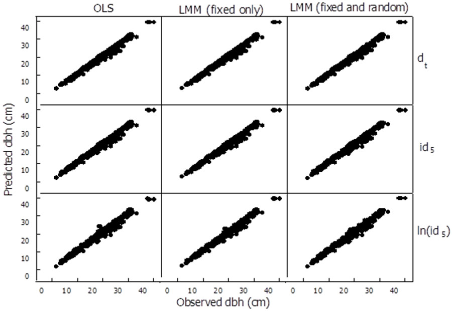
Additionally, the best OLS and LMM models for each response variable, based on AIC, were also evaluated in their capability to predict dbh of P. occidentalis five years after initial measurement using the independent validation data set. To accomplish this evaluation we first examined the correspondence expected between observed and predicted future diameter on the 9 different dbh growth models tested (Fig. 1). The rows on the chart depict three models for each of the response variables (the future diameter dt, diameter increment id5 and natural log of diameter increment ln(id5), respectively). The columns correspond to the three statistical techniques explored (ordinary least squares, linear mixed effect models considering only the fixed effects part and linear mixed effect models considering both the fixed and random effects of the model). Although the scale in the chart is small, it can be clearly seen that there is more noise in the bottom row corresponding to the natural log of diameter increment [ln(id5)] models, than in the first row (future diameter dt models).
Fig. 1 - Comparison of observed vs. predicted five-year future diameter for 9 different dbh growth models. The first row were models using future dbh (dt) as the dependent variable, second row using 5-year diameter increment (id5) as the dependent variable, and bottom row using natural logarithm of 5-year diameter increment [ln(id5)] as the dependent variable. Model parameter estimates of predictor variables for each dependent variable were fitted using ordinary least squares (OLS column 1), linear mixed models including only the fixed effects (LMM column 2) and linear mixed models including both fixed and random effects (LMM column 3).
Continuing with the evaluation on the best OLS and LMM, we performed the proposed analysis on goodness-of-fit statistics on the best six model formulations. The results are presented on Tab. 4. The dt model (eqn. 12) had better goodness-of-fit statistics when it was evaluated using the independent data set. It performed better in five out of seven statistics, although the margin of difference was narrow. Average error was under 5% (1 cm) over 5 years, and percent bias was less than 3%. The d5 model fitted by LMM corresponded reasonably well with the validation data, with a RMSE = 1.037 cm. Model from eqn. 12 produced on average smaller residuals, ranging from 0.00 to 0.45 cm in the validation data set, and MSE ranged from 0.22 to 1.70 cm2.
Tab. 4 - Goodness-of-fit statistics for best six models predicting diameter at breast height (dbh) five years after initial measurement using an independent validation data set of 200 trees. Models had different response variables and parameter estimation techniques (OLS and LMM, described in text). (dt): future dbh at time t; (id5): 5-year diameter increment; ln(id5+0.01): natural logarithm of 5-year diameter increment. (*): see text for descriptions.
| Goodness- of-fit statistics* |
Response Variable | ||||||||
|---|---|---|---|---|---|---|---|---|---|
| d t | id 5 | ln(id5+0.01) | |||||||
| OLS | LMM | OLS | LMM | OLS | LMM | ||||
| Fixed | Fixed & Random | Fixed | Fixed & Random | Fixed | Fixed & Random | ||||
| MSE | 2.265 | 2.273 | 2.175 | 2.222 | 2.22 | 2.115 | 2.397 | 2.311 | 2.226 |
| RMSE | 1.505 | 1.508 | 1.475 | 1.491 | 1.49 | 1.454 | 1.548 | 1.52 | 1.492 |
| RMSE% | 6.868 | 6.881 | 6.732 | 6.803 | 6.8 | 6.637 | 7.066 | 6.939 | 6.81 |
| BIAS | 0.083 | 0.076 | 0.104 | 0.13 | 0.072 | 0.132 | -0.069 | -0.036 | -0.053 |
| BIAS% | 0.378 | 0.346 | 0.477 | 0.594 | 0.329 | 0.601 | -0.317 | -0.165 | -0.24 |
| MAD | 0.863 | 0.853 | 0.81 | 0.819 | 0.814 | 0.749 | 0.869 | 0.836 | 0.801 |
| R 2 | 0.951 | 0.951 | 0.953 | 0.952 | 0.952 | 0.954 | 0.948 | 0.95 | 0.952 |
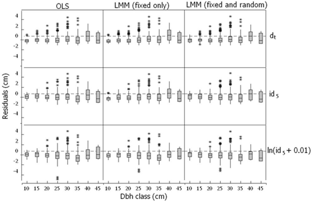
To check for dependencies or systematic trends throughout the range of diameter classes, we proceeded to plot the residuals vs. predicted five-year diameter increment estimated with models with fixed and fixed plus random prediction in that order for the top row; fixed and fixed plus random prediction in the middle row; and fixed and fixed plus random prediction in the bottom row. The residuals did not exhibit dependencies or systematic trends; although the box and whiskers plot (Fig. 2) shows more narrow boxes for the top row which corresponds to model from eqn. 12, throughout the diameter classes. In general, model from eqn. 12 fitted by LMM slightly underestimates the diameter five years after initial measurement in all diameter classes.
Fig. 2 - Residuals vs. predicted five-year diameter increment estimated with models with fixed and fixed plus random prediction in that order for the top row; fixed and fixed plus random prediction in the middle row; and fixed and fixed plus random prediction in the bottom row.
Discussion
Diameter growth and yield prediction is one of the primary components of individual-tree growth models. These models allow detailed analyses on stand structure, but need additional equations to describe other components (e.g., tree mortality and recruitment) of tree or stand growth to make a complete stand or tree projection system. Diameter increment of P. occidentalis was studied as a stochastic process where a fixed part of a model explains the population-average increment, and a random component captures tree-to-tree variability. The study compares two statistical techniques, stepwise OLS regression and mixed models; two approaches, future diameter and diameter increment; and several classes of independent variables for predicting future diameter of P. occidentalis in La Sierra, Dominican Republic.
The best model was evaluated based on the seven goodness-of-fit statistics. Between the alternatives, the linear mixed model which included, for prediction purposes, both fixed and random effects was superior to just employing the fixed part of the LMM and ordinary least squares models. Modeling diameter through time as response variable was superior to the other two response variables, namely five-year diameter increment and its log transformation. The former resulted in a better fit, especially in regards to MSE, RMSE, RMSE% and R2.
To detect prediction anomalies, one-to-one correspondence between observed vs. future predicted dbh were plotted in Fig. 2. No conspicuous anomalies were noted. The proposed formulation can be considered a projection model, containing a fixed part which explains the mean value for the future diameter and the unexplained residual variability is described by including random parameters. Model from eqn. 12 produces logical predictions of future dbh, and by means of differentiation, dbh increment is easily obtained. The fixed components of model from eqn. 12 included initial tree size, elapsed time and BAL as explanatory variables. Future diameter of a tree increased by approximately 4% on average for every centimeter added to initial dbh. Time contributed on average to 1% increment to the dbh reached five years hence.
Tree size is a good indicator of future growth, reflecting past competitive status and different genetic responses to the environment ([19], [3]). With model from eqn. 12, diameter increment increased by a factor of 0.0903 for each unit increase in initial diameter. The positive sign associated with the parameter estimate of this variable may be a reflection of the low densities characterizing the studied plots. Previous results from density management trials in the study region have reported that for P. occidentalis stands older than 18 years of age, similar to those used in this study, the optimum residual density should be 700 trees per hectare (TPH). In our study, the number of stems per hectare varied from 192 to 950, with 11 stands having at most 470 TPH, which is roughly 67% of the desired residual density. Seven stands were between 78 and 96%, and four were slightly above 100% of the target residual density.
Variables commonly used to quantify competition and site productivity in individual tree diameter growth models, such as the number of trees per ha ([28]), stand density index, basal area per hectare ([30]) and site index ([18]) were also tested in all the models evaluated. However, they were not significant in our best fitting model. Most surprisingly is the lack of predictive ability of site index, particularly since diameter increment appeared to be lowest in those stands geographically located along the dryer portion of the study region (1000 mm of average annual rainfall). These stands were also characterized by having very shallow sandy soils with depth between 30 and 50 cm. Locations where diameter increment was larger, soil depth was between 80 and 100 cm and the average annual precipitation ranged from 1200 to 1600 mm. It appears that height development for this species is not a good proxy for site productivity.
As basal area of larger trees (BAL) increases, competition increases and that leads to a reduction in the diameter growth. That was manifested in the present study with the negative coefficient for this predictor variable. An increase of one unit in BAL decreased future diameter by 0.2%, on average. P. occidentalis is an intolerant species that needs direct sunlight to grow at full potential. Basal area of larger trees is considered a variable that captures one-sided competition for light ([3]). The stands studied were not crowded so the competition for light was not that severe and is reflected in the biologically logical but moderate influence of BAL on diameter growth.
The R matrix in the model from eqn. 12 indicates significant random variability among trees. This suggests that other tree variables may need to be considered in the model. In terms of variability, model from eqn. 12 detected larger quantities between trees (0.355) than between plots (0.049). Pukkala ([21]) attributes this phenomenon to human error in diameter increment measurement. In our case, the reason behind this pattern of variability may be found on the disparate arrangement of densities among the stand studied. These results are consistent with the findings of Palahí et al. ([18]) when modeling growth for Pinus silvestrys L. in northeast Spain and contrary to the findings of Calama & Montero ([7]) for Pinus pinea, also in Spain.
Application of the fixed and random part of the model results in slightly biased estimates (less than 0.45 cm) of the future diameter for trees larger than 40 cm. For trees up to 28 cm, biased is less than 0.10 cm. In the validation dataset, 97% of the total variability in projected future diameter was explained by model from eqn. 12.
In Tab. 3, we explored the effects of the covariates included in model from eqn. 12. It remains unclear whether inclusion of random effects is an improvement over adding additional appropriate predictor variables. The presence of BAL in the model decreased the values from the G and R matrices by 92 and 4 percent, respectively (Tab. 2). AIC and BIC values are decreased by about 2%. Comparing model predictions using independent validation data demonstrated that all the models had moderately improved fit statistics when random effects were included in the evaluation. The degree of improvement behaved in a similar manner for most fit statistics, with differences in the range of values for MSE, RMSE and RMSE% of 0.53, 0.23 and 1.05, respectively. The absolute difference between the extreme values for bias and relative bias (%) in all the models was 0.20 and 0.92. The differences in values for MAD were only 0.15 and R2 values were practically equivalent. This might be due to the fact that most of the sites are relatively poor, and the models may be capturing a gradual deceleration in growth, even for the short time period represented by the data. Slow growth was noticed during the first few remeasurements, with little or no growth in the last. Some considerations can be hypothesized as responsible for the absence of growth.
Differences in the performance of the mixed and fixed models in individual tree growth and yield modeling have been reported by others. Adame et al. ([1]), working with Quercus pyrenaica Willd, found that most of the variability in tree growth occurred at the within-stand level, rather than between stands. Uzoh & Oliver ([26]) reported that the best relationship between five-year periodic annual diameter increments of ponderosa pine trees was provided by linear mixed models. Other authors ([7], [18]) have considered random variability in modeling diameter increment. They reported increase improvement in the fitting process when mixed models including both fixed and random parameters were employed.
Within-stand variability could be the result of the density of the stands under study. Basal area per hectare varied from 9.3 to 31.3 m2 ha-1, with 7 stands having less than 15 m2 ha-1, 9 stands having between 15 and 20 m2 ha-1 , 6 stands between 20 and 25 m2 ha-1, and three stands with more than 25 m2 ha-1. Stands with lower density have more space and resources available for tree growth. Even though it was tested, stand basal area was not a significant predictor variable in model from eqn. 12. Perhaps its effect is being captured by the random part of the model.
Conclusions
We have determined that linear mixed models are the best statistical technique to fit linear regression models, for predicting dbh over time in P. occidentalis trees in La Sierra, Dominican Republic. The proposed future diameter model from eqn. 12 prevailed over five-year diameter increment as the more appropriate response variable to model for predicting future dbh, using variables related to tree size such as initial dbh (d0), elapsed time (t), and variables related to competition like the cumulative basal area of the trees larger than subject tree (BAL0) as predictor variables. Model from eqn. 12 does not depend on age or distance. The final predictor variables were selected based on their ecological importance to tree growth and on fitting statistics. Simulations performed with model from eqn. 12 showed that coefficients for predictor variables were biologically appropriate. Specifically, larger trees (d0) grew faster, trees growing in stands having higher densities (TPH0) grow slower, and increasing levels of competition at the tree level (BAL0) also decreased predicted future diameter.
Based on Akaike’s Information Criterion and the Bayesian’s Information Criterion, the most appropriate covariance structures was the unstructured (UN). The adequacy of the covariance structure was confirmed by the likelihood ratio test which was statistically significant (p < 0.0001). Evidence reported in Tab. 3 shows that the linear mixed models tested produced better fit statistics when plots were considered as random effects. This confirms our expectations that the inclusion of fixed plus random effects was more effective than including only fixed effects in the predictions of future dbh.
This study is the first attempt to model individual tree growth of P. occidentalis in the Dominican Republic. Model evaluation is an uninterrupted course of action, and the results from this study can be further improved in the immediate future. For the moment, the model will enable estimation of diameter on individual P. occidentalis trees in the north central portion of Cordillera Central, for up to five years in the future, based on information regarding initial dbh and basal area of trees within stands. The species has great economic, ecological and social importance, and model from eqn. 12 can provide valuable information for decision-makers, forest managers and researchers. It is biologically consistent according to forest growth expectation, but projections longer than 5 years should be avoided until validation of the model using longer term data becomes available. The model should be simple to apply and can be used to facilitate and ensure the sustainable management of P. occidentalis.
Acknowledgements
We want to express our gratitude to Drs. Ralph D. Nyland, Lianjun Zhang and Edwin H. White for reviewing and suggesting their valuable inputs. Funding for this project was provided by the J. William Fulbright Foreign Scholarship Board (FSB), and by the Graduate Assistantship program at the State University of New York, College of Environmental Science and Forestry and the Collegiate Science and Technology. Major contributions were received from the Dominican government through Ministerio de Educacion Superior Ciencia y Tecnologia and its funding program (FONDOCYT). We also like to thank the Program on Latin America and the Caribbean at Syracuse University (PLACA), Cooperativa San José, Plan Sierra Inc., and PROCARYN.
References
Gscholar
Gscholar
Gscholar
Gscholar
Gscholar
Gscholar
Gscholar
Gscholar
Gscholar
Gscholar
Gscholar
Gscholar
Gscholar
Gscholar
Gscholar
Gscholar
Gscholar
Gscholar
Gscholar
Authors’ Info
Authors’ Affiliation
Vicerrectoria de Investigaciones e Innovación, Pontificia Universidad Catolica Madre y Maestra, Santiago de los Caballeros (Dominican Republic)
College of Environmental Science and Forestry, State University of New York, 1 Forestry Drive, 13210 Syracuse, NY (USA)
Corresponding author
Paper Info
Citation
Bueno-López S, Bevilacqua E (2013). Diameter growth prediction for individual Pinus occidentalis Sw. trees. iForest 6: 209-216. - doi: 10.3832/ifor0843-006
Academic Editor
Marco Borghetti
Paper history
Received: Oct 26, 2012
Accepted: Mar 06, 2013
First online: May 27, 2013
Publication Date: Aug 01, 2013
Publication Time: 2.73 months
Copyright Information
© SISEF - The Italian Society of Silviculture and Forest Ecology 2013
Open Access
This article is distributed under the terms of the Creative Commons Attribution-Non Commercial 4.0 International (https://creativecommons.org/licenses/by-nc/4.0/), which permits unrestricted use, distribution, and reproduction in any medium, provided you give appropriate credit to the original author(s) and the source, provide a link to the Creative Commons license, and indicate if changes were made.

Web Metrics
Breakdown by View Type
Article Usage
Total Article Views: 74795
(from publication date up to now)
Breakdown by View Type
HTML Page Views: 64074
Abstract Page Views: 3950
PDF Downloads: 5296
Citation/Reference Downloads: 24
XML Downloads: 1451
Web Metrics
Days since publication: 4735
Overall contacts: 74795
Avg. contacts per week: 110.57
Article Citations
Article citations are based on data periodically collected from the Clarivate Web of Science web site
(last update: Mar 2025)
Total number of cites (since 2013): 6
Average cites per year: 0.46
Publication Metrics
by Dimensions ©
Articles citing this article
List of the papers citing this article based on CrossRef Cited-by.
Related Contents
iForest Similar Articles
Research Articles
Estimating biomass of mixed and uneven-aged forests using spectral data and a hybrid model combining regression trees and linear models
vol. 9, pp. 226-234 (online: 21 September 2015)
Research Articles
Site quality assessment of degraded Quercus frainetto stands in central Greece
vol. 8, pp. 53-58 (online: 12 May 2014)
Research Articles
Individual-based approach as a useful tool to disentangle the relative importance of tree age, size and inter-tree competition in dendroclimatic studies
vol. 8, pp. 187-194 (online: 21 August 2014)
Research Articles
Total tree height predictions via parametric and artificial neural network modeling approaches
vol. 15, pp. 95-105 (online: 21 March 2022)
Research Articles
Assessment of age bias in site index equations
vol. 9, pp. 402-408 (online: 11 January 2016)
Research Articles
Analyzing regression models and multi-layer artificial neural network models for estimating taper and tree volume in Crimean pine forests
vol. 17, pp. 36-44 (online: 28 February 2024)
Research Articles
Integrating area-based and individual tree detection approaches for estimating tree volume in plantation inventory using aerial image and airborne laser scanning data
vol. 10, pp. 296-302 (online: 15 December 2016)
Research Articles
Nonlinear mixed model approaches to estimating merchantable bole volume for Pinus occidentalis
vol. 5, pp. 247-254 (online: 24 October 2012)
Research Articles
Relationship between environmental parameters and Pinus sylvestris L. site index in forest plantations in northern Spain acidic plateau
vol. 9, pp. 394-401 (online: 16 January 2016)
Research Articles
Local neighborhood competition following an extraordinary snow break event: implications for tree-individual growth
vol. 7, pp. 19-24 (online: 14 October 2013)
iForest Database Search
Search By Author
Search By Keyword
Google Scholar Search
Citing Articles
Search By Author
Search By Keywords
PubMed Search
Search By Author
Search By Keyword


