
Analyzing regression models and multi-layer artificial neural network models for estimating taper and tree volume in Crimean pine forests
iForest - Biogeosciences and Forestry, Volume 17, Issue 1, Pages 36-44 (2024)
doi: https://doi.org/10.3832/ifor4449-017
Published: Feb 28, 2024 - Copyright © 2024 SISEF
Research Articles
Abstract
The taper and merchantable tree volume equations are the most used models in forestry because of their accuracy in estimating both total and merchantable tree volume. However, numerous studies reported that artificial neural network models show fewer errors and a greater success rate as compared to regression models. This study used data from 200 Crimean pine trees in Turkey’s Central Anatolia and Mediterranean Region to assess the performance of artificial neural network (ANN) models and the Max-Burkhart’s equation for estimating taper and merchantable tree volume. The most accurate results were obtained using 3 hidden layers and 10 neurons in the taper model and 1 hidden layer and 100 neurons in the volume model. The hyperbolic tangent sigmoid function was used for the ANN analysis and hyper-parameter customization. Using the ANN model with hyper-parameter customization, the AAE in the Max-Burkhart taper model decreased from 9.315 to 6.939 (-25.5%), the RMSE decreased from 3.072 to 2.656 (-13.5%), and the FI increased from 0.964 to 0.966 (+1.23%). Similarly, using the ANN model with hyper-parameter customization, the AAE in the Max-Burkhart volume model decreased from 0.056 to 0.013 (-76.6%), the RMSE decreased from 0.247 to 0.12 (-51.6%), and the FI increased from 0.909 to 0.979 (+7.69%). Our results showed that the ANN models’ predictions were more accurate and reliable compared to the Max-Burkhart’s equations. We resolved overfitting via hyper-parameter modification, which also allowed for monitoring the impact of error and prediction outputs at various learning rates. It was also possible to develop tree taper and volume equations with lower error rates in both training and validation data, consistent with tree growth trends in both data sets.
Keywords
Compatible Tree Taper, Merchantable Volume Equations, Crimean Pine, Multilayer Artificial Neural Network, Hyper-parameter Customization
Introduction
The estimation of the growing stock is very important for the best forest management and the optimization of derived products ([5]). Single-tree traits measurements like diameter at breast height (DBH), total tree height (TTH), and volume are critical in forest inventory studies ([21]). Accurate estimation of merchantable tree volume is essential for long-term sustainability, management of growing stock resources, operational forestry, and scientific research ([18]). For these reasons, it is crucial to accurately calculate the volume of single trees, both in the context of forestry inventory and in the scope of scientific study.
Forest managers are required to determine the volume of standing trees that can be marketed without logging. To this aim, many methods (single or double-entry tree volume tables, yield tables, etc.) have been suggested and used to estimate merchantable tree volume ([21]). However, the individual tree volume cannot be determined directly using analytical methods since the tree stem that makes up the merchantable tree volume does not precisely reflect known geometric shapes such as cylinder, paraboloid, cone, or niloid ([21], [46]). Allometric models are often used to estimate the total tree volume (TTV), considering the DBH (d1.3 m) and the total height of the trees ([4]). However, according to Tang et al. ([45]), these models cannot estimate TTV up to any height limit or saleable quantities up to any height or diameter restriction. Foresters should also make estimations of the stem diameter at various heights along the bole for predicting the variety of wood products ([6]), and taper equations have been well-developed to solve such problems. Taper equations do not only describe the stem shapes but also provide the estimation of various wood product types and assortments, such as the merchantable volume or individual volume for logs between two different heights ([16]). When used in combination with actual volume prediction systems, these equations also provide volume predictions at the dominant height limit and throughout the entire tree height ([18], [22]).
Taper equations have long been studied in forestry research, and can be divided into two general classes. In the first group of equations, the tree shape is represented as a single continuous function ([26], [16], [18]). The second group of equations (segmented polynomial taper equations - SPTEs) calculates the TTV using different models for different parts of the tree stem, such as the niloid, cylinder, paraboloid, and cone ([23]). Using a relative diameter or height function, volume ratio equations can predict merchantable volume as a percentage of the TTV ([45]). SPTE models were introduced by Max & Burkhart ([23]), using a separate polynomial for each different shape segment of the tree and then combines these polynomials into a single model.
Hierarchical measured data are used to make conic equations. These data structures can cluster or differentiate among them, even though they come from trees with different properties ([8], [33]). One of the most widespread statistical problems, data auto-correlation (i.e., interdependence of data) may arise from this situation ([19]). The effect of a measurement performed at any location on the tree stem on the following diameter measurement value should be analyzed in such hierarchical data structures. Hierarchical data structures are a prevalent issue in forestry research, and they may contradict the idea of data independence, which is one of the fundamental assumptions in regression analysis. Furthermore, the autocorrelation problem in hierarchical data structures can reduce the reliability of the model by introducing a systematic error in the confidence intervals of the parameter estimates in tapered merchantable volume models ([17], [8]). As a consequence, regression models with decreasing estimation reliability may produce erroneous estimates ([48]).
In hierarchical data structures, when data independence cannot be established and there is a correlation problem between the data, a variance-covariance matrix allowing the structure to be modeled is used. For this purpose, the use of autoregressive modeling approaches ([12]) or nonlinear mixed effect models ([20]), which reduce the negative effect of many observations in single trees on the predictions, may come into prominence in forest literature.
Nonlinear regression modeling is a generally accepted and widely applied technique. However, it has significant limitations, such as the need to make assumptions about normality and homogeneity, the requirement for defining the form of the fitting function, and the need of accurate initial values for correct parameter estimates in nonlinear models. These characteristics are looked for in the construction of forecasting models. In contrast, ANN models can develop knowledge using experience without making any assumptions about the form of the fitting function. Additionally, the relationships between input and output variables are built into link weights of the network ([30]). Haykin ([14]) identified the three main attributes of ANNs: nonlinearity, excitability, and inter-neuronal interaction.
ANNs have several advantages over traditional modeling methods because they do not require statistical assumptions like traditional regression modeling, as well as their ability to detect complexity in the computational process, thus allowing for non-linear relationships between input and output variables ([37]). Many studies in forestry have applied ANN models ([9], [10], [29]), which have been proved to obtain more accurate predictions than regression models ([1], [42]). Because of the above advantage, there has been a shift in recent years from the use of traditional regression models to ANNs, particularly in growth and yield modeling research ([13], [31], [40]). ANNs have also been used for predicting single tree and stand characteristics such as tree volume ([30], [24]) and tree taper ([7], [27]), especially in recent years. The use of ANN models is increasing due to the inadequacy of traditional regression models in taper prediction and their autocorrelation problem. Moreover, the ability to model both taper and merchantable volume at the same time makes ANNs more advantageous than traditional regression models.
However, ANN models have also some disadvantages, among which the most important are the “underfitting” and “overfitting” problems. Indeed, ANN models with complicated architectures may perform well on the training dataset but poorly on new, independent datasets. Numerous studies on forest development modeling have demonstrated that using the more effective nonlinear modeling characteristics of deep learning network models can solve the problem of “underfitting”. On the other hand, overfitting predictions in ANN models is a common problem in forestry. The overfitting problem can lead to predictions in taper and merchantable volume models without any biological meaning. For example, ANN models might not assess the right relationships between diameter and volume or growth trends for trees. According to Ercanli et al. ([11]), this problem can be solved by customizing the hyper-parameters used to build ANN topologies. Although the adaptive learning rate of ANN models is maintained constant in many studies, a “learning rate customization” can be applied which addresses the process of locating the optimum prediction for various learning rates. In this study, different hyper-parameter options are tested, including 10 hidden layers, 5 neurons, and a learning rate of 19. This adds up to 950 multilayer ANN model options. Changing the learning rate during the training stage of the appropriate ANN model will help finding the best model with biological meaning, thereby solving the overfitting problem of ANN modeling.
The purpose of this study was to develop taper and volume equation systems for stem diameters and merchantable stem volume estimation in Crimean pine (Pinus nigra J.F. Arnold subsp. pallasiana [Lamb.] Holmboe) stands in the Central Anatolian and Mediterranean regions of Turkey. We compared how well multilayer ANN methods and SPTE models by Max & Burkhart ([23]) can predict taper and TTV. We also investigated how changing hyperparameters in ANN model structures can help get rid of overfitting and show how error changed for different learning rates while getting rid of overfitting.
Material and methods
Material
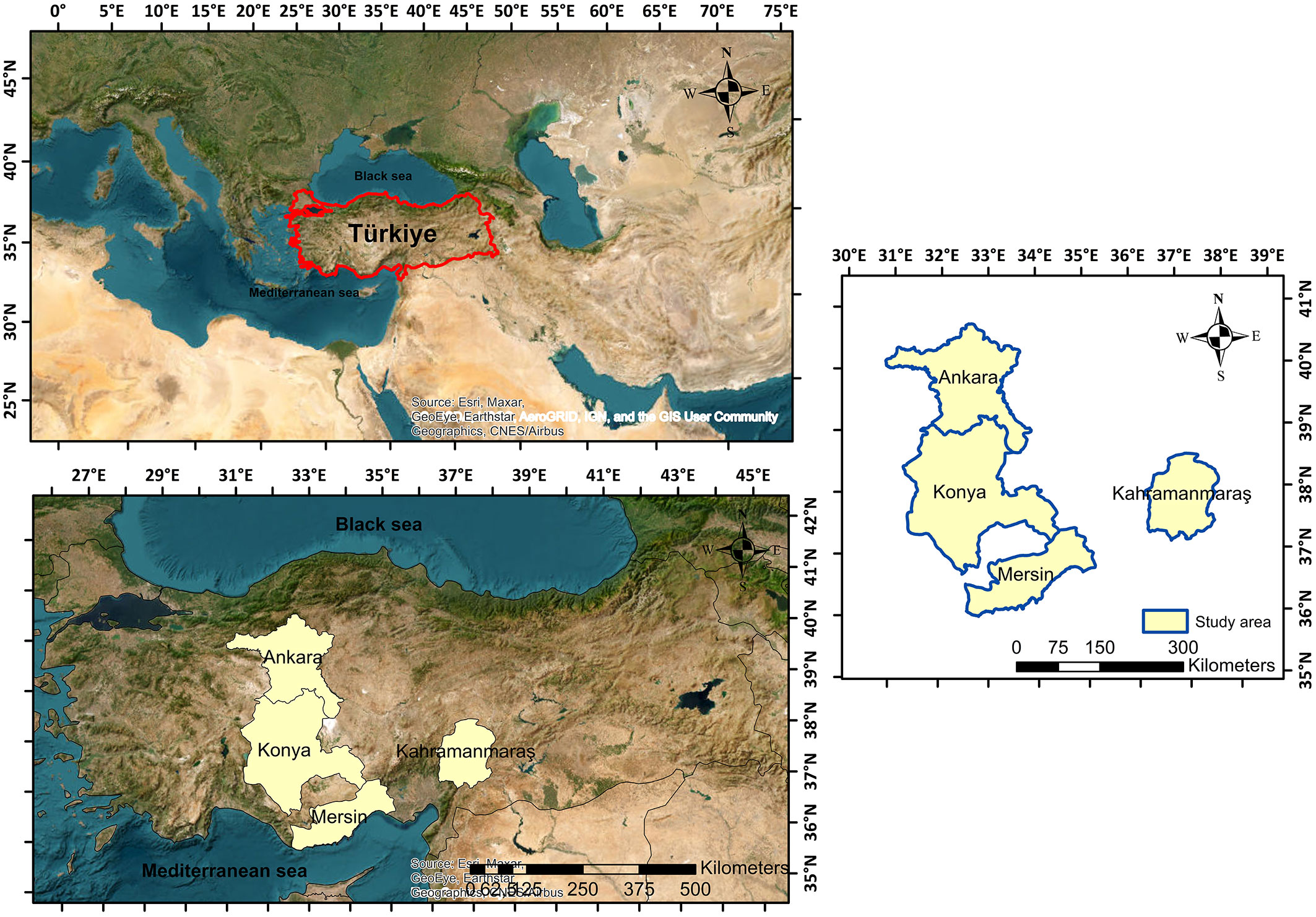
The study was conducted on Crimean pine trees from pure stands located in several Turkish provinces which represent important ecosystem areas for this species, namely Uluhan/Nallihan (Ankara - 31°21′ N, 40°11′ E), Andirin (Kahramanmaras - 37°19′ N, 36°12′ E), Asagiçigil/Ilgin (Konya - 39°56′ N, 31°84′ E), and Alahan/Mut (Mersin - 39°56′ N, 32°51′ E - Fig. 1). Due to its geographical location, geological structure, and climate variation, Turkey has an extensive and diverse flora, with over 11.000 taxa distributed over the country. Crimean pine is the second most widespread coniferous tree species in Turkey after red pine and is the dominant tree species in the study areas. The study provinces of Nallihan and Asagiçigil present a continental climate, while Andirin and Alahan provinces show Mediterranean climate characteristics. The mean elevations of the study stands in the above provinces are 755, 1100, 1300, and 300 m a.s.l., respectively; the mean annual temperatures are 11.7, 12.6, 11.8, and 19.2 °C; and the mean annual precipitations are 390, 1370, 260, and 370 mm, respectively; the slope ranged between 10% and 70%.
Fig. 1 - The study area.
The sampled trees were randomly selected from the study area and sampled with a distribution which reflects the variation in diameter and height classes and the variation in TTV as well. A total of 200 sample trees were cut from the stump height (0.3 m), the stump diameter was recorded, and the other stem diameters over bark were measured at 1-meter intervals (1.3, 2.3, 3.3, …, m above the ground) up to the tree’s top. These sample trees were divided into two groups: training (model) data (170 trees, 85% of total data) and validation data (30 trees, the remaining 15%). Tab. 1 shows some descriptive statistical values for the sampled trees.
Tab. 1 - Descriptive statistics of the fitting and validation datasets. (STD): standard deviation.
| Dataset | N | Variables | Min | Max | Mean | STD |
|---|---|---|---|---|---|---|
| Fitting | 170 | DBH (cm) | 11.0 | 60.0 | 31.4053 | 11.0561 |
| TTH (m) | 5.64 | 24.0 | 12.7274 | 4.1566 | ||
| TTV (m3) | 0.0414 | 3.1185 | 0.6603 | 0.6084 | ||
| Validation | 30 | DBH (cm) | 13.9 | 58.0 | 33.0633 | 13.5006 |
| TTH (m) | 7.27 | 23.0 | 13.445 | 5.0439 | ||
| TTV (m3) | 0.0792 | 2.9595 | 0.8148 | 0.8027 |
The TTV was calculated by adding the volumes of the stump log, the sections, and the crown for each sample tree. The stump was supposed to be cylindrical, but the top section was assumed to be cone-shaped. Smalian’s formula (eqn. 1) was used to compute the volume of each section; the cylinder formula (eqn. 2) was used to calculate the stump volume; and the cone formula (eqn. 3) was used to calculate the top volume:
where d0 is the thick diameter of the tree, d0.3 is the stump diameter, and dn is the thin diameter of the tree. The addition of the calculated volume for each section yielded the TTV.
SPTE and taper-based volume prediction
It is assumed in the SPTE that the tree stem can be separated into three geometric shapes. The top section of the tree resembles a cone, the stem part resembles a paraboloid, and the bottom log part has a nyloid shape ([23]). SPTEs contain a different equation for each component of the tree stem, and thus they can explain the variation in trunk shapes quite successfully. In this study we used the SPTE to describe the variations in stem forms with two joining points (eqn. 4):
where Z = h/H, Ii = 1 if Z ≤ ai and Ii=0 if Z > ai. In all equations, d is the diameter over bark at height h (cm), D is the diameter at breast height over bark (cm), h is the height at the measurement point (above ground along the stem, in m), H is the total tree height (TTH, m), a1 and a2 are join points to be estimated from the sample data for the Max & Burkhart ([23]) equation, and b1-b4 are regression coefficients.
Integrating the results obtained from eqn. 4 in the following merchantable volume equation ([49] - eqn. 5):
where w = h/H. A TTV equation was derived by setting h = H (eqn. 6):
The constant-form factor volume equation has a specific instance in eqn. 6 ([44]). A series of algebraically compatible taper and volume equations is given by eqns. 4-6.
The PROC MODEL function of the SAS® statistical package ([39]) was used to predict the parameter estimates and other statistical criteria for the Max & Burkhart’s taper equation. The iteration of seemingly unrelated regression (ITSUR) parameters has also been added to reduce the error variance of volume data when using the PROC MODEL function to estimate the segmented taper model. The ITSUR technique and the MODEL procedure of the SAS/ETS® statistical program ([39]) were used to simultaneously harmonize the components of the system.
Autoregressive modeling for stem diameter estimates
Various degrees of autoregressive modeling are recommended solve the serial correlation problem that may occur in taper predictions ([45], [34]). Some refinements were made to the Max & Burkhart ([23]) taper equation ([8]) to account for autocorrelation, using a modified continuous autoregressive error structure (CAR(1)). The PROC MODEL was used in SAS® for the Max & Burkhart ([23]) taper equation to add the continuous autoregressive error structure (CAR(1)) to the parameter estimation steps when the autoregressive modeling method was used ([8]).
To account for first-order autocorrelation and increase the error terms, the following CAR(1) model form was used ([50] - eqn. 7):
where eij is the j-th ordinary residual of the i-th individual (i.e., the difference between the observed and the estimated diameters of the i-th tree at height measurement j), d1 = 1 for j > 1, and d1 = 0 for j = 1, is the first-order continuous autoregressive parameter to be estimated, and hij > hij-1 is the distance separating the j-th from the j-th - 1 observation within each tree, hij > hij-1. The ρ1 parameter was expanded in the following way using dummy variables to account for the position of the measurements along the bole: ρ1 + ρ11d11 + ρ12d12, where d11 and d12 are either 1 or 0, depending on the relative position of the measurements. Before accounting for autocorrelation, the relative positions of each model were graphically evaluated. Finally, the correlations between the raw residuals and the residuals from previous observations within each tree for the relative height classes were calculated.
ANNs for taper and TTV estimates
In this study, we applied ANNs for predicting the diameter along the bole and individual TTV. ANNs is one of the artificial intelligence (AI) methods which emulates the human nerve cell and the data transfer process that takes place in these cells. ANNs are developed in a structure consisting of three layers: the “input layer”, “hidden layer”, and the “output layer”. In particular, if the number of intermediate layers is increased, complex network models with a higher number of layers than the three-layer basic structure of ANN models can be obtained. The layered structure of ANN models has 5 basic elements: inputs, weights, summation functions, activation functions, and outputs ([28]). The activation function, which connects various layers, can be changed by the user who connects the network model and conducts the network training.
The 3-layers network structure depends on the ANN model used in the training of data. The connections between these layers are regulated by some parameters, such as the hyperbolic tangent (tanh), the rectifier, and the maxout, etc, which serve as transition functions between the input and hidden layers and the hidden and output layers. Preliminary evaluations carried out in the present study suggested that several activation functions, such as the rectifier and the maxout, resulted in significantly poor TTV projections. As a consequence, the tanh function ranging from -1 to 1 was chosen as an activation function to train the ANNs as it provided the best predictions of TTV. The number of neurons in the intermediate layer is another crucial issue in ANN models, and their number can be established by the user. Both the type of activation function and the number of neurons are important parameters that affect the accuracy of predictions in the ANN model ([25]).
In this study, the measured stem diameters (in cm) of the sample trees (170 trees in the training dataset) were defined as the output variable (target variable) in the training of ANN models. In addition, the DBH of trees, TTH, and other independent variables from Max & Burkhart ([23]) were taken as input variables for training ANN models. Several ANN models were trained to predict both the diameter along the bole and the TTV of the sampled trees. In the latter model the TTV of trees was set as the output variable, and the DBH and the TTH were taken as input variables. We use the Levenberg-Marquardt algorithm and ANN based on multilayer feedforward backpropagation networks to calculate SPTE and TTV. The number of hidden layers in the model was ranging from 1 to 10 (1-, 2-, 3-, 4-, 5-, 6-, 7-, 8-, 9-, and 10-layer numbers), and a customized, multi-layer model training has been obtained. In addition, five different neuron options (10, 30, 50, 70, and 100) were considered for hidden layers for the training of ANN models.
A unique feature of this study is the special focus on eliminating overfitting problems and violations of biological realism in SPTE and TTV. Overfitting is a common issue in forestry when estimating various individual tree and stand properties ([11], [3]) which can cause ANN models to be very effective for their own training datasets but very unsuccessful when tested on independent datasets.
ANN modeling in forestry must take into account the biological realism of the model predictions, as extensively discussed in the literature ([2], [47], [35]). In this study, we aimed both to limit the overfitting issue of ANN models and to maintain the biological realism of the their predictions through the application of hyper-parameterized values in the model structure. To this end, several preliminary analyses were carried out to identify the hyper-parameters to be used in the network topology. Hyper-parameters such as moment rate and early stopping with root mean squared error (RMSE) showed poor ability in solving the overfitting problem. In contrast, hyper-parameters such as learning rate successfully predicted taper, total and merchantable tree volume by avoiding overfitting. Nineteen different learning rates in the range 0-1 were tested in the model (from 1 × 10⁻⁶ up to 0.1), and the multi-layered ANN model training was conducted using the above learning rate values. Overall, a total of 950 multi-layer ANN models were trained and their performance evaluated in this study (10 different numbers of hidden layers × 5 different numbers of neurons × 19 different learning rate options).
When training all hyper-parameterized ANN models, the “h2o.deeplearning” function of the H2O package in R was used to predict tree tapers, total and merchantable volumes ([15]). The H2O package was selected as it offers quick and easy network model training for numerous hyper-parameterized variables and used to train multi-layer feedforward neural networks.
Evaluations of SPTE and TTV models
To compare and evaluate the predictive accuracy of equations obtained with Max & Burkhart ([23]) taper equation, TTV equation, and ANN models with hyper-parameter customizations, various statistical fitting criteria were used, such as the average absolute error (AAE - eqn. 8), RMSE (eqn. 9), RMSE% (eqn. 10), Akaike information criterion (AIC - eqn. 11), Bayesian information criterion (BIC - eqn. 12), and the fit index (FI - eqn. 13):
where y = TTVi or di, n is the number of data points, and k is the number of inputs of the independent variable in the prediction methods within the model.
Here, observed and predicted values are related to stem diameters and TTV, since in this study prediction models were developed for both taper and TTV. Therefore, these statistical fitting criteria were calculated and evaluated separately for both equations.
Results
The goodness-of-fit statistics (AAE, RMSE, RMSE%, FI, AIC, and BIC) obtained for all the developed models are presented in Tab. 2 (for taper) and Tab. 3 (for TTV) for the training data set, and Tab. 4 (for taper) and Tab. 5 (for TTV) for the validation data set.
Tab. 2 - Goodness-of-fit statistics for taper prediction in the training dataset. (BPHP); Best Predictive Hyper-Parameter; (ANN - HPC): ANN model without hyper-parameter customization; (SPTE): the SPTE of Max & Burkhart ([23]) based on CAR(1).
| No. Hidden Layers |
No. of Neurons |
BPHP Value |
AAE | RMSE | RMSE% | AIC | BIC | FI |
|---|---|---|---|---|---|---|---|---|
| 1 | 30 | 0.02 | 6.8024 | 2.6124 | 10.8383 | 1177.6207 | 2858.1273 | 0.9583 |
| 2 | 30 | 0.01 | 7.3046 | 2.7072 | 11.1685 | 1221.0043 | 2901.5108 | 0.9552 |
| 3 | 10 | 0.02 | 6.7272 | 2.5979 | 10.6424 | 1170.8512 | 2851.3577 | 0.9588 |
| 4 | 50 | 0.005 | 7.4139 | 2.7273 | 11.2757 | 1230.0442 | 2910.5508 | 0.9546 |
| 5 | 30 | 0.005 | 7.3328 | 2.7124 | 11.0405 | 1223.3507 | 2903.8573 | 0.9551 |
| 6 | 70 | 0.003 | 7.1661 | 2.6814 | 11.0882 | 1209.3444 | 2889.8510 | 0.9561 |
| 7 | 70 | 0.003 | 7.3871 | 2.7224 | 10.9900 | 1227.8458 | 2908.3523 | 0.9547 |
| 8 | 50 | 0.003 | 7.5689 | 2.7557 | 11.1161 | 1242.6516 | 2923.1581 | 0.9536 |
| 9 | 30 | 0.005 | 7.1406 | 2.6766 | 11.1263 | 1207.1772 | 2887.6838 | 0.9562 |
| 10 | 50 | 0.005 | 7.5262 | 2.7479 | 11.2888 | 1239.2010 | 2919.7076 | 0.9539 |
| ANN - HPC | 5.3375 | 2.3131 | 9.4983 | 1027.4250 | 2359.5350 | 0.9673 | ||
| SPTE | 9.9693 | 3.1613 | 12.8715 | 1407.9020 | 2740.0120 | 0.9389 | ||
Tab. 3 - Goodness-of-fit statistics for TTV prediction in the training dataset. (BPHP); Best Predictive Hyper-Parameter; (ANN - HPC): ANN model without hyper-parameter customization; (SPTE): the SPTE of Max & Burkhart ([23]) based on CAR(1).
| No. Hidden Layers |
No. of Neurons |
BPHP Value |
AAE | RMSE | RMSE% | AIC | BIC | FI |
|---|---|---|---|---|---|---|---|---|
| 1 | 100 | 0.02 | 0.0102 | 0.1017 | 15.4102 | -384.5554 | -270.7204 | 0.9722 |
| 2 | 70 | 0.01 | 0.0109 | 0.1049 | 15.8405 | -379.2664 | -265.4314 | 0.9704 |
| 3 | 10 | 0.03 | 0.0112 | 0.1066 | 16.0097 | -376.5140 | -262.6789 | 0.9695 |
| 4 | 100 | 0.01 | 0.0119 | 0.1096 | 16.9441 | -371.8345 | -257.9995 | 0.9677 |
| 5 | 100 | 0.005 | 0.0121 | 0.1108 | 16.9376 | -369.9668 | -256.1317 | 0.9670 |
| 6 | 10 | 0.01 | 0.0122 | 0.1112 | 16.6813 | -369.4435 | -255.6085 | 0.9668 |
| 7 | 70 | 0.003 | 0.0141 | 0.1194 | 18.6085 | -357.3231 | -243.4881 | 0.9617 |
| 8 | 30 | 0.01 | 0.0136 | 0.1171 | 17.4638 | -360.5637 | -246.7287 | 0.9632 |
| 9 | 100 | 0.005 | 0.0142 | 0.1197 | 18.6124 | -356.9199 | -243.0848 | 0.9615 |
| 10 | 50 | 0.005 | 0.0130 | 0.1148 | 17.6664 | -364.0099 | -250.1749 | 0.9646 |
| ANN -HPC | 0.1681 | 0.4124 | 59.6382 | -146.5630 | -32.7280 | 0.5431 | ||
| SPTE | 0.0402 | 0.2018 | 39.5826 | -268.0990 | -154.2640 | 0.8907 | ||
Tab. 4 - Goodness-of-fit statistics for taper prediction in the validation dataset. (BPHP); Best Predictive Hyper-Parameter; (ANN - HPC): ANN model without hyper-parameter customization; (SPTE): the SPTE of Max & Burkhart ([23]) based on CAR(1).
| No. Hidden Layers |
No. of Neurons |
BPHP Value |
AAE | RMSE | RMSE% | AIC | BIC | FI |
|---|---|---|---|---|---|---|---|---|
| 1 | 30 | 0.02 | 6.7499 | 2.6212 | 10.3706 | 227.7038 | 535.7790 | 0.9670 |
| 2 | 30 | 0.01 | 8.4257 | 2.9285 | 11.6023 | 252.9841 | 561.0592 | 0.9588 |
| 3 | 10 | 0.02 | 6.9385 | 2.6575 | 10.4494 | 230.8447 | 538.9198 | 0.9661 |
| 4 | 50 | 0.005 | 8.2732 | 2.9019 | 11.4537 | 250.9016 | 558.9767 | 0.9595 |
| 5 | 30 | 0.005 | 7.9231 | 2.8398 | 11.0515 | 245.9731 | 554.0483 | 0.9612 |
| 6 | 70 | 0.003 | 8.2638 | 2.9002 | 11.4709 | 250.7728 | 558.8479 | 0.9596 |
| 7 | 70 | 0.003 | 7.6382 | 2.7883 | 10.7244 | 241.7988 | 549.8740 | 0.9626 |
| 8 | 50 | 0.003 | 8.1375 | 2.8780 | 11.1287 | 249.0175 | 557.0926 | 0.9602 |
| 9 | 30 | 0.005 | 7.5987 | 2.7811 | 11.0231 | 241.2073 | 549.2824 | 0.9628 |
| 10 | 50 | 0.005 | 8.9094 | 3.0114 | 11.8665 | 259.3479 | 567.4231 | 0.9564 |
| ANN - HPC | 87.5046 | 9.4165 | 31.8548 | 517.2830 | 761.7660 | 0.5720 | ||
| SPTE | 9.3150 | 3.0723 | 11.6957 | 261.9150 | 506.3990 | 0.9544 | ||
Tab. 5 - Goodness-of-fit statistics for TTV prediction in the validation dataset. (BPHP); Best Predictive Hyper-Parameter; (ANN - HPC): ANN model without hyper-parameter customization; (SPTE): the SPTE of Max & Burkhart ([23]) based on CAR(1).
| No. Hidden Layers |
No. of Neurons |
BPHP Value |
AAE | RMSE | RMSE% | AIC | BIC | FI |
|---|---|---|---|---|---|---|---|---|
| 1 | 100 | 0.02 | 0.0133 | 0.1195 | 14.6496 | -59.7242 | -42.9298 | 0.9786 |
| 2 | 70 | 0.01 | 0.0146 | 0.1249 | 15.3228 | -58.4095 | -41.6151 | 0.9766 |
| 3 | 10 | 0.03 | 0.0180 | 0.1390 | 17.4086 | -55.1908 | -38.3964 | 0.9710 |
| 4 | 100 | 0.01 | 0.0169 | 0.1345 | 16.9094 | -56.1845 | -39.3901 | 0.9729 |
| 5 | 100 | 0.005 | 0.0177 | 0.1375 | 17.1662 | -55.5216 | -38.7272 | 0.9717 |
| 6 | 10 | 0.01 | 0.0141 | 0.1228 | 14.9751 | -58.9189 | -42.1244 | 0.9774 |
| 7 | 70 | 0.003 | 0.0215 | 0.1519 | 19.3320 | -52.5308 | -35.7364 | 0.9654 |
| 8 | 30 | 0.01 | 0.0208 | 0.1492 | 18.7324 | -53.0795 | -36.2851 | 0.9667 |
| 9 | 100 | 0.005 | 0.0212 | 0.1505 | 19.0802 | -52.8052 | -36.0108 | 0.9660 |
| 10 | 50 | 0.005 | 0.0200 | 0.1462 | 18.5912 | -53.6742 | -36.8798 | 0.9680 |
| ANN - HPC | 0.5330 | 0.7557 | 166.9549 | -4.4040 | 12.3910 | 0.1443 | ||
| SPTE | 0.0569 | 0.2469 | 38.3476 | -37.9690 | -21.1740 | 0.9087 | ||
As for taper estimations, the ANN model with hyper-parameter customization (with 10 neurons, 3 hidden layers, and 0.02 learning rate values) had an AAE value of 6.7272, RMSE of 2.5979, RMSE% of 10.6424, AIC of 1170.8512, BIC of 2851.3577, and FI value 0.9588 (Tab. 2). Similar to the values in the training dataset, the validation dataset yielded prediction results with AAE = 6.9385, RMSE = 2.6575, RMSE% = 10.4494, AIC = 230.8447, BIC = 538.9188, and FI = 0.9661 (Tab. 4). The goodness-of-fit statistics showed that the ANN model with customized hyper-parameters performed better than all the other estimation methods on the validation data set (Tab. 4) in terms of AAE, RMSE, RMSE%, AIC, BIC error values, and FI.
The ANN model with hyper-parameter customization (100 neurons, 1 hidden layer, and 0.02 learning rate values) had the best predictive capacity, with AAE = 0.0102, RMSE = 0.1017, RMSE% = 15.4102, AIC = -384.5554, BIC = -270.7204, and FI = 0.9722 for the training data set (Tab. 3). Similarly, for the validation dataset, this ANN model showed the most accurate prediction with 0.0133 AAE, 0.1195 RMSE, 14.6496 RMSE%, -59.7242 AIC, -42.9298 BIC, and 0.9786 FI.
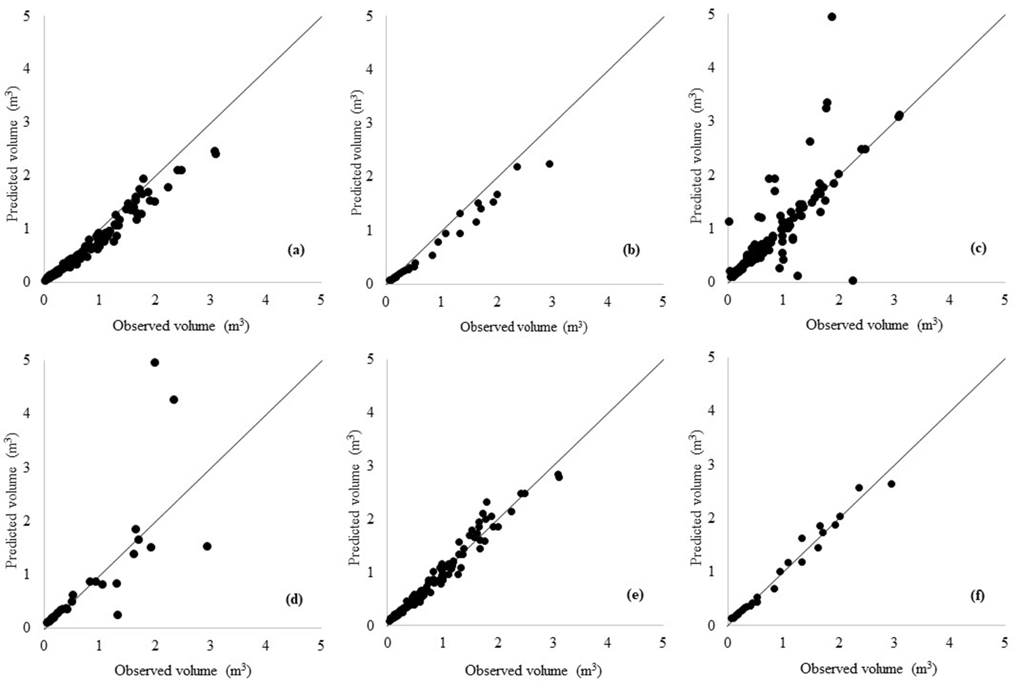
The scatter plots of taper and TTV estimates vs. the actual volume values obtained by all models are well dispersed along the 1:1 line (Fig. 2, Fig. 3).
Fig. 2 - Scatterplots of predicted vs. observed diameter of training data (a: Max-Burkhart; c: ANN without hyper-parameter customization; e: ANN with hyper-parameter customization) and predicted vs. observed diameter of validation data (b: Max-Burkhart; d: ANN without hyper-parameter customization; f: ANN with hyper-parameter customization) for taper equations.
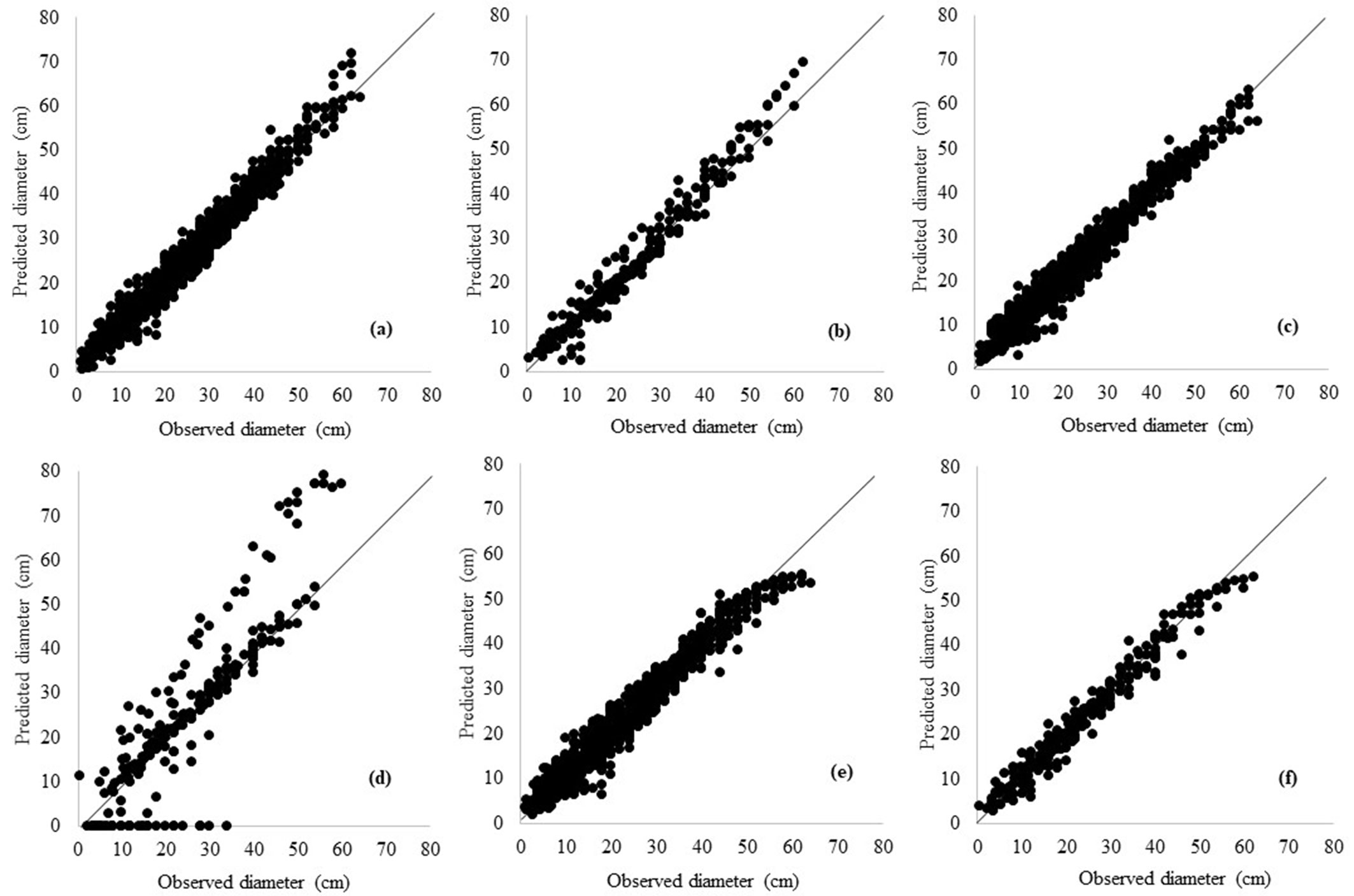
Fig. 3 - Scatterplots of predicted vs. observed volume of training data (a: Max-Burkhart; c: ANN without hyper-parameter customization; e: ANN with hyper-parameter customization) and predicted vs. observed volume of validation data (b: Max-Burkhart, d: ANN without hyper-parameter customization, f: ANN with hyper-parameter customization) for TTV equations.
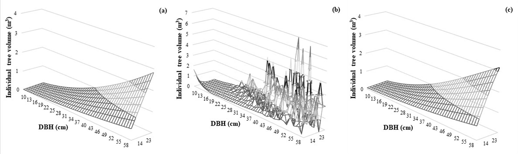
We fixed the overfitting problem of the ANN models and used the training data set to obtain the TTV prediction graphics for each method, along with the biologically realistic fit or violation conditions (Fig. 3). The TTV plot made by the Max-Burkhart model looked like a real biological system (Fig. 3a), but the TTV plot made by the ANN model without hyper-parameter customization showed a TTV development predicted as a wavy line with peak formation (Fig. 3b). However, the ANN model with hyper-parameter customization fixes this issue (Fig. 3c).
Discussion
In this study, Crimean pine taper and TTV in the Central Anatolia and Mediterranean regions of Turkey were predicted using two different modeling methods and the hyper-parameter customization in ANN modeling. The performance of the superior ANN models in various layers and with various numbers of neurons was also compared (Tab. 2, Tab. 3). The ANN’s model structure was customized, the estimation scenarios for several learning rates were examined and evaluated, and the best learning rate was determined. We also examined an extensive variety of scenarios from the most basic to the most complex architectures (up to 10 hidden layers and 100 neurons) and solved the overfitting issue.
While overfitted models may give good results on the training dataset, they may underperform using the validation dataset ([11]). Also, it is worth noting that ensuring the reliability of ecological models is crucial to guaranteeing their accuracy. To this end, we fixed the overfitting problem likely affecting our initial ANN models, as it could be argued by the very high values of AAE, RMSE, RMSE%, AIC, BIC, and FI. Indeed, predictions based on these error measures may appear accurate even if they are not.
Although the ANN method initially provided more accurate results than the Max and Burkhart model (Tab. 4), overfitting of the data was evident and could not be resolved (Fig. 3b). Therefore, the hyper-parameter customization recommended by Ercanli et al. ([11]) was used and the accuracy of model predictions using different learning rates was monitored. Not only the overfitting was resolved after the analyses with the adaptive rate disabled, but there was also an obvious reduction in model errors and a higher FI.
Our results showed that the ANN method seems to perform better than other methods for both taper and TTV models both in terms of FI and RMSE% (Tab. 2, Tab. 4). This method may also produce models that are biologically meaningful for the expected TTV growth by setting up a sigmoid trend with a known asymptote. The results of ANN models with violations of biological realism can also be trained with other parameter adjustments. Our results confirmed the findings by Ercanli et al. ([11]), who considered the hyperparameters customization as a useful way to obtain the most accurate results, with lower error rate than other methods, and in line with biological realism (Fig. 3). Consequently, taper and TTV can be effectively estimated using ANN methods.
Taper equations have been widely used in many inventory studies because they can provide detailed TTV estimation using easily measurable variables such as diameter and height. ANNs worked better than traditional regression methods in many studies, including those that developed taper, volume, diameter, and height equations or estimated leaf area index ([30], [32], [27], [36], [9], [10], [41], [43], [38]). However, in many of these studies the learning rates were left at their default values, and overfitting was not taken into account in the ANN model development.
The results of this study support previous results that the ANN method outperforms the traditional regression method. Additionally, monitoring for changes in various learning rates and the customization of the model structure helped solving both overfitting of the training dataset and the biological realism of predictions in the validation dataset (Fig. 4).
Fig. 4 - Three-dimensional graphs of training data. (a): Max-Burkhart; (b): ANN without hyper-parameter customization; (c): ANN with hyper-parameter customization) for TTV equations.
Conclusion
Taper and TTV equations for Crimean pine were developed by eliminating the autocorrelation problem using both the traditional regression method and the ANN method. The structure of the ANN model network was changed to adapt to biological growth through changing the learning rate and/or applying a customized hyper-parameterization of the models. The variance in errors according to the different learning rates included in the models was also monitored, confirming the superior performances of ANN-based procedures over conventional regression models.
ANN methods do not require statistical assumptions and can provide predictions at least as good as or even better than traditional regression methods. Moreover, hyper-parameter (e.g., learning rate) customization allows to overcome the problem of data autocorrelation. According to our results, the ANN models with hyper-parameter customization outperformed the traditional regression methods in predicting the taper and TTV of Crimean pine in Turkey, thus providing results that meet the needs of decision-makers and practitioners in the management of forest resources. However, it is worth stressing that the results of this study should not be extrapolated outside the study area unless adequate tests of the developed models are carried out.
Acknowledgments
The author thanks Uluhan, Andirin, Asagiçigil, and Alahan Forest Management Directorates and their staff for their support in the preparation of this research.
References
Gscholar
Gscholar
Gscholar
Gscholar
Gscholar
Gscholar
Gscholar
Gscholar
Gscholar
Gscholar
Authors’ Info
Authors’ Affiliation
Artvin Çoruh University, Faculty of Forestry, 08100, Artvin (Turkey)
Corresponding author
Paper Info
Citation
Sahin A (2024). Analyzing regression models and multi-layer artificial neural network models for estimating taper and tree volume in Crimean pine forests. iForest 17: 36-44. - doi: 10.3832/ifor4449-017
Academic Editor
Rodolfo Picchio
Paper history
Received: Aug 14, 2023
Accepted: Jan 04, 2024
First online: Feb 28, 2024
Publication Date: Feb 29, 2024
Publication Time: 1.83 months
Copyright Information
© SISEF - The Italian Society of Silviculture and Forest Ecology 2024
Open Access
This article is distributed under the terms of the Creative Commons Attribution-Non Commercial 4.0 International (https://creativecommons.org/licenses/by-nc/4.0/), which permits unrestricted use, distribution, and reproduction in any medium, provided you give appropriate credit to the original author(s) and the source, provide a link to the Creative Commons license, and indicate if changes were made.

Web Metrics
Breakdown by View Type
Article Usage
Total Article Views: 827
(from publication date up to now)
Breakdown by View Type
HTML Page Views: 214
Abstract Page Views: 207
PDF Downloads: 387
Citation/Reference Downloads: 0
XML Downloads: 19
Web Metrics
Days since publication: 59
Overall contacts: 827
Avg. contacts per week: 98.12
Article Citations
Article citations are based on data periodically collected from the Clarivate Web of Science web site
(last update: Feb 2023)
(No citations were found up to date. Please come back later)
Publication Metrics
by Dimensions ©
Articles citing this article
List of the papers citing this article based on CrossRef Cited-by.
Related Contents
iForest Similar Articles
Research Articles
Compatible taper-volume models of Quercus variabilis Blume forests in north China
vol. 10, pp. 567-575 (online: 08 May 2017)
Research Articles
Modelling taper and stem volume considering stand density in Eucalyptus grandis and Eucalyptus dunnii
vol. 14, pp. 127-136 (online: 16 March 2021)
Research Articles
The use of tree crown variables in over-bark diameter and volume prediction models
vol. 7, pp. 132-139 (online: 13 January 2014)
Research Articles
Modeling compatible taper and stem volume of pure Scots pine stands in Northeastern Turkey
vol. 16, pp. 38-46 (online: 22 January 2023)
Research Articles
A geographically weighted deep neural network model for research on the spatial distribution of the down dead wood volume in Liangshui National Nature Reserve (China)
vol. 14, pp. 353-361 (online: 27 July 2021)
Research Articles
Nonlinear mixed model approaches to estimating merchantable bole volume for Pinus occidentalis
vol. 5, pp. 247-254 (online: 24 October 2012)
Research Articles
Allometric equations to assess biomass, carbon and nitrogen content of black pine and red pine trees in southern Korea
vol. 10, pp. 483-490 (online: 12 April 2017)
Research Articles
Coupling daily transpiration modelling with forest management in a semiarid pine plantation
vol. 9, pp. 38-48 (online: 06 August 2015)
Research Articles
Total tree height predictions via parametric and artificial neural network modeling approaches
vol. 15, pp. 95-105 (online: 21 March 2022)
Research Articles
Identification of wood from the Amazon by characteristics of Haralick and Neural Network: image segmentation and polishing of the surface
vol. 15, pp. 234-239 (online: 14 July 2022)
iForest Database Search
Search By Author
Search By Keyword
Google Scholar Search
Citing Articles
Search By Author
Search By Keywords
PubMed Search
Search By Author
Search By Keyword


