Comparing image-based point clouds and airborne laser scanning data for estimating forest heights
iForest - Biogeosciences and Forestry, Volume 10, Issue 1, Pages 273-280 (2017)
doi: https://doi.org/10.3832/ifor2077-009
Published: Feb 23, 2017 - Copyright © 2017 SISEF
Research Articles
Abstract
Accurate and updated knowledge of forest tree heights is fundamental in the context of forest management. However, measuring canopy height over large forest areas using traditional inventory techniques is laborious, time-consuming and excessively expensive. In this study, image-based point clouds produced from stereo aerial photographs (AP) were used to estimate forest height, and compared to Airborne Laser Scanning (ALS) data. We generated image-based Canopy Height Models (CHM) using different image-matching algorithms (SGM: Semi-Global Matching; eATE: enhanced Automatic Terrain Extraction), which were compared with a pure ALS-derived CHM. Additionally, plot-level height and density metrics were extracted from CHMs and used as explanatory variables for predicting the Lorey’s mean height (LMH), which was measured at 296 reference points on the ground. CHMSGM and CHMALS showed similar results in predicting LMH at sample plot locations (RMSE% = 8.54 vs. 7.92, respectively), while CHMeATE had lower accuracy (RMSE% = 13.23). Similarly, CHMSGM showed a lower normalized median absolute deviation (NMAD) from CHMALS (0.68 m) compared to CHMeATE (1.1 m). Our study revealed that image-based point clouds using SGM in the presence of high-resolution ALS-derived digital terrain model (DTM) provide comparable results with ALS data, while the performance of image-based point clouds using eATE is poorer than ALS for forest height estimation. The findings of this study provide a viable and cost-effective option for assessing height-related forest structural parameters. The proposed methodology can be usefully applied in all those countries where AP are updated on a regular basis and pre-existing historical ALS-derived DTMs are available.
Keywords
Forest Inventory, Canopy Height Model, Stereo Aerial Photographs, LiDAR, Semi-Global Matching (SGM), enhanced Automatic Terrain Extraction (eATE)
Introduction
Measuring forest height using traditional forest inventory techniques is laborious, time-consuming and excessively expensive for large forest areas ([5], [39]), whereas with remote sensing (RS), single stands and large areas can be covered cost-efficiently ([24]).
Forest canopy height models (CHMs) and their derived metrics can be used for a variety of valuable application in forest science. For instance, CHM can be used for change detection, canopy gap dynamic, and single tree detection ([32], [49], [17], [50]). Height and density metrics derived from CHMs at plot level can be used for the assessment of forest height, forest timber volume, biomass, basal area and mean diameter-at-breast-height point (DBH) using the area-based approach (ABA - [1], [25], [30], [34], [40], [45]). The same parameters at single tree level can also be derived directly (i.e., tree height and crown area) or indirectly (i.e., volume, basal area and mean DBH) from CHM by separation of individual crown using the individual tree detection approach (ITD - [2], [12], [17]). CHM as well as height metrics derived from Airborne Laser Scanning (ALS), also called Light detection and ranging (LiDAR) data, were successfully applied in many case studies for the assessment of forest structure information, as ALS has the capability for extraction of both the digital terrain model (DTM), which represents the forest floor, and the digital elevation model (DEM), which represents the entire canopy of forest ([28], [29], [13], [31], [42], [46], [48]).
Over the last decade, ALS has revolutionized the process of forest mapping and has been used operationally for forest inventory in many Nordic countries like Norway, Finland, and Sweden ([22], [26], [27]). However, in many countries, ALS acquisitions are often not as frequently updated as digital stereo aerial photographs (AP) by the survey administrations, and therefore cannot be used for the regular measurement as needed for forest management planning due to high cost. It is also unclear in most federal states in Germany, the time frequency of ALS data acquisition ([3]). APs are updated on a routine basis at regular time intervals by the survey agencies/administration ([40], [39], [47]). As an example in the Baden-Württemberg state of Germany, APs are regularly updated every three years by the Landesamt für Geoinformation und Landentwicklung (LGL) and can be used for the regular update of forest structure information, while ALS acquisitions are not that consistent over time. Since ALS data is considered more accurate, we have used it as one of the reference datasets in our study to estimate forest heights, despite its high costs.
Automatic process of AP based on image matching algorithms can provide sufficiently dense and highly accurate image-based 3D point clouds for the generation of DSM, but the generation of DTM in a dense forest environment, where forest floor is not visible is challenging ([45]). Hence, the limiting factor of the image-based point clouds is the vertical penetration, which is provided by ALS. Thus the idea of combining photogrammetric image-based DSM with pre-existing historical ALS DTM could be a promising solution for the generation of CHM ([36], [38], [15], [43], [1]).
With the recent advancements of modern stereo photogrammetry, one of the most active research areas in computer vision for 3D mapping is stereo image matching ([37]). There are several software packages and image matching algorithms for the generation of 3D point clouds. For our study, we have selected two widely used programs that are based on different methodological approaches. One is enhanced Automatic Terrain Extraction (eATE): an ERDAS LPS module, that is a normalized correlation area based search windows approach for the identification of corresponding pixels using spatial correlation metrics. The search range along the epipolar line is constrained by estimated minimum and maximum elevation values ([41]). The second one is Semi-Global Matching (SGM) developed by Hirschmüller ([9], [10]). It uses a pixel-wise approach, utilizing the radiometric robust mutual information and a smoothness constraint to generate dense surface point clouds. The method first identifies a pixel on the base image and then seeks for the similar pixel along the epipolar line in the pair image. The minimum aggregated cost leads to a disparity map. Several studies showed that SGM is the superior methodology ([9], [6], [35]). So far, comparative studies between the point clouds image matching algorithms have not focused over forest terrain, and this forms the main research gap for our study. Our specific goals were: (a) to assess the performance of the images-based point clouds in comparison with ALS for estimating forest heights; (b) to identify which of the two widely used image matching algorithms, namely SGM and eATE, is best suited for forest height retrieval.
Material and methods
Study area and field data
The study area is located in a relatively flat area north of Karlsruhe in the Federal State of Baden-Württemberg, Germany, extending from 49° 03′ 37.302″ N and 08° 24′ 02.846″ E to 49° 01′ 18.773″ N and 08° 25′ 49.981″ E (Fig. 1). The total area covers 12 km2 and the dominant forest tree species are Scots pine (Pinus sylvestris L.), European/Common beech (Fagus sylvatica L.), Sessile oak (Quercus petraea leibel.) and Red oak (Quercus rubra L.). Further tree species including Douglas fir (Pseudotsuga menziesii), Norway spruces (Picea abies) and European larch (Larix decidua) can also occur occasionally.
Fig. 1 - Geographical location of the study site. The green points represents the location of the reference sample plots on the ground, while the yellow rectangular block delineates the small subset area where a transect (yellow line) was drawn for visual comparison of the CHMs. Orthophoto and aerial photos: © Landesamt für Geoinformation und Landentwicklung für Baden-Württemberg (⇒ http://⇒ www.lgl-bw.de) Az.: 2851.9-1/3.
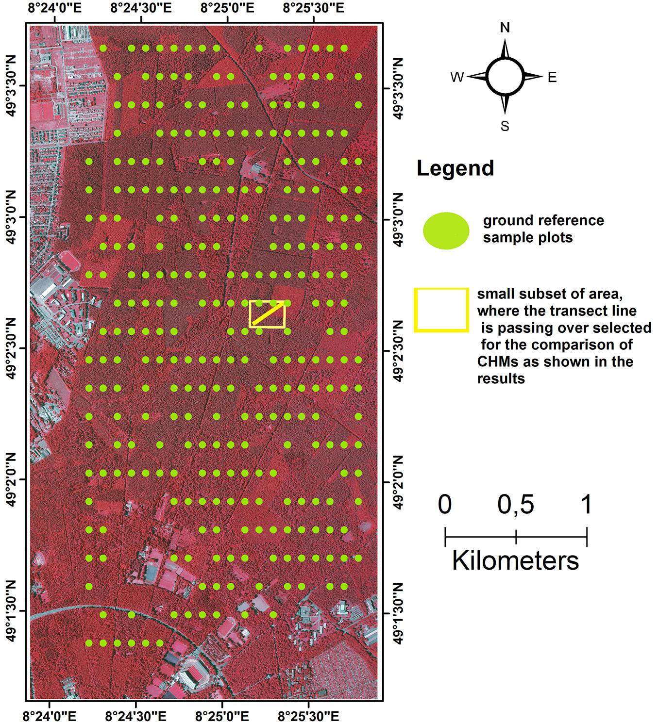
The state forest service of Baden-Württemberg set up a total of 296 permanent circular concentric plots during the summers of 2006 and 2007 over the entire study area, and these have been used for the collection of ground reference data (Fig. 1). The sample plots were distributed systematically over the study area in a 100 × 200 m sample grid. On each plot, trees with diameter-at-breast-height (DBH) <10 cm, between 10 and 15 cm, between 15 and 30 and >30 cm were measured, if they were exactly at the distance of 2, 3, 6 and 12 m from the plot center. Two dominant heights of each main tree species and one dominant height of other mixed species were measured. The remaining tree heights were predicted by species-specific stand height curves developed by the Forest Research Institute, Baden-Württemberg (FVA), Germany ([18]). Finally, ground Lorey’s mean height (LMH) was calculated by multiplying the tree height (h) by its basal area (g), and then the sum of the multiplication of individual heights and basal areas are divided by the sum of the plot basal area ([20] - eqn. 1):
where LMH is the ground Lorey’s mean height, g is the basal area and h is the tree height. We selected LMH since it is a standard forest measure to characterize forest canopy height, giving higher weights to trees with a larger basal area.
Remote sensing data
Full-waveform ALS data was acquired in 2009 by Milan Geoservice Gmbh using the IGL Litemapper 5600 system with a Riegl LMS-Q560 (240 kHz) scanner. For the summer 2009 acquisitions during leaf-on conditions, the study area was flown over twice to obtain a high point density. The first flight was conducted in north-south and the second in the east-west direction. The details of the flight and system parameters of ALS are shown in Tab. 1.
Tab. 1 - Details of flight and system parameters of Airborne Laser Scanning (ALS).
| Parameters | Value |
|---|---|
| Flying height [m] (above ground level) |
600 |
| Field of view [deg] (full scan angle) |
60 |
| Strip width [m] | 520 |
| Measurement rate [kHz] | 240 |
| Point density [points m-2] | ~ 22 |
| Flying velocity [m s-1] | 46 |
Similarly, we used a block of 28 APs with four spectral bands (blue, green, red and near-infrared). The APs were acquired in summer 2009 during the leaf-on canopy conditions. The aero-triangulation was done by Landesamt für Geoinformation und Landentwicklung (LGL) with ground control points and based on initial measurement by Global Navigation Satellite System (GNSS) and inertial measurement unit (IMU) (LGL). For the projection of the generated datasets, DHDN/3 Gauss-Krüger coordinate system was used throughout the process. More details about the technical parameters are given in Tab. 2.
Tab. 2 - Details of flight and technical characteristics of Digital Stereo Aerial Images.
| Details | Stereo aerial photographs /images (AP) |
|---|---|
| Camera | UltraCamXP |
| Flying height | 2950 m |
| Image overlap | 60% & 30% |
| Swat width | 520 m |
| Acquisition date | Summer 2009 |
| No. of images used in a block | 28 |
| Spectral bands | blue, green, red and near-infrared |
| Resolution (GSD) | 0.2 m (20 cm) |
Generation of image-based point clouds using enhanced Automatic Terrain Extraction (eATE) and Semi-Global Matching (SGM)
Image-based point clouds were generated from AP using eATE manager (integrated module in the LPS ERDAS IMAGINE 2015) by choosing a point sampling density of 1, whereby every other pixel is matched. A point sampling density of zero might be useful in term of accuracy, but it takes a considerable longer period to be processed ([4]), and hence was not used. A pixel block size of 100 was selected where eATE engine divides the images into blocks of pixels and processes each block separately. Thread 2 indicates the number of distributed processing threads for this eATE process and each thread is assigned to a separate core in the machine. The radiometry threshold defines the measurement (percentage) of contrast around the central pixel in the master image. The default is 2.5, and it is recommended to use larger (than 2.5) threshold for high contrast images, thereby ensuring a higher possibility of getting good correlated points. For low-contrast images, it is recommended to use a smaller threshold so that eATE correlates more points regardless of the contrast. If the threshold is set to zero then all points will be matched ([4]). For segmentation, we used the infrared band because of its higher sensitivity to vegetation compared to the other bands. During the correlation process, we optimized the matching by using all available spectral bands. For window size, which is representative of the pixel area used for computing the correlation coefficient between left and right images, we chose a larger (15×15) value. While the default value is 9×9, it is recommended to use a larger window size for areas with minimal variation (right in our case) and a smaller window (e.g., 5×5) for areas with greater topographic relief. Coefficient start and end indicates the correlation coefficient used for each pyramid level. Higher coefficients range (0.7-0.8) produces higher accuracies, but fewer points may be matched, while a lower range increases the number of correlated points. The search window is the maximum search size in pixels surrounding the point to be interpolated and has a square shape. The default value is 50; a higher number is suitable for low contrast areas, while a lower number is recommended for areas with higher contrast. We use a higher value because it gives better points despite increasing the processing time. A low value may give more uniformly distributed points, but the points may not be accurate. Standard deviation tolerance indicated the tolerance (in meters) for determining the standard deviation of the planar fit (default = 3) and LSQ refinement indicated the pyramid level to apply a least squares refinement. Edge contrast represents the number of pyramid levels to apply edge constraint, and tolerance means the measure in pixel used to accept or reject the point during reverse matching. Smoothing looks for spikes in elevation, and low smoothing option ensures a minimal smoothing for data with few anomalies ([4]).
Similarly, image-based point clouds were generated from AP using SGM XPro (integrated in LPS ERDAS IMAGINE 2015) by setting urban situation to zero, as it can be applied to urban areas. We selected Keep vertical which retains point clouds on the vertical surfaces like trees tops.
Generation of Digital Surface Model (DSM) and Digital Terrain Model (DTM)
DSMs with a spatial resolution of 1 m were calculated from the image-based point clouds using eATE (DSMeATE) and SGM (DSMSGM). Similarly, DSMALS and DTMALS were generated from ALS data. For the generation of DSMs and DTMs the active filtering and interpolation techniques as implemented in the TreesVis software ([44]) were used. In TreesVis, the generation of DSM and DTM from point clouds is done by using an “Active Surface Filtering Algorithm”. Before starting the iterative process, the algorithm created three surfaces: the “active surface, a “punch surface” and a “mask surface”. The active surface is only allowed to move vertically up and down. Moreover, the active surface represents the desired output, whether DSM or DTM is to be generated. In the case of DTM generation, the active surface is placed lower than the punch surface and move upward, while in the case of DSM generation the active surface is placed above the punch surface and move downward. Each pixel of the punch surface is filled with height values of the lowest 3D point for the calculation of DTM. Similarly, the highest 3D point is chosen as a height for the punch surface for the calculation of DSM within pre-defined pixel size spatial resolution. The mask surface is automatically filled with special flags, necessary for the regulation of minimization process. After creation of these surfaces, the original 3D point clouds were no longer needed for minimization and could be deleted. However, for visualization purposes, the point clouds are still present in the random access memory (RAM) of the computer. The developed active algorithm was up to now only allowed to move up and down, which simplified the process to a great extent. The reason for the movement and deformation of active surface are two types of forces, i.e., the inner forces and the outer forces. The iterative process continues until these forces reach the level of equilibrium. The inner forces introduce stiffness in the active surface in such a way that it will not touch each detail of the punch surface. Each pixel of the active surface is influenced by the expansion, which is defined by the distance to the eight neighboring pixels. The outer forces attract the active surface, which brings deformity in the active surface. The relation between the inner and outer forces defined the degree of deformity. Two different forces are used as outer forces, i.e., a “pressure force” which pushes the active surface downward in case of DTM generation and upward in case of DSM generation. The second outer force is the magnetic ones, where each pixel of the punch surface is attracting the active surface toward itself. The magnetic force is always positive. The iteration process will stop until the vertical movement is lower than a pre-defined threshold. The uncritical pre-defined threshold was set to 0.01 [m], which is better than the vertical measurement accuracy of the given 3D points.
Calculation of Canopy Height Models (CHMs) and computation of explanatory variables (metrics)
We generated three kinds of canopy height models: (1) CHMSGM by subtraction of DTMALS from DSMSGM; (2) CHMeATE by subtraction of DTMALS from DSMeATE; and (3) CHMALS by subtraction of DTMALS from DSMALS.
The most commonly used ALS and image-based derived metrics from CHMs or point cloud in forest inventory are the percentiles ([25]). A total of 15 height metrics were calculated from each CHM, i.e., maximum, minimum, mean and the height percentiles (h99, h95, h90, h80, …, h10). For variation and heterogeneity of forest canopy height, we calculated the coefficient of variation (CV) and standard deviation (SD) from each CHM. As mentioned above, the metrics were derived from the vertical distribution of CHMs using a 12-meter radius circle, which corresponds to the size of ground sample plots. Besides, we calculated the canopy cover density parameters and Canopy Volume (CVol) which takes into account the horizontal distribution of the canopy structure. We calculated the forest canopy density (cd) by dividing the number of pixels with heights above 2 m by the total number of pixels within an area of 12 m radius circular sample plots. Besides, we derived ten types of forest cover density metrics (i.e., cd1, cd2, cd3, …, cd10) at sample plots location followed by the methodology adopted by Naesset ([25]), Rahlf et al. ([34]) and Straub et al. ([40]). The range between the lower canopy height (>2m) and maximum height was divided into ten fractions of equal length. Each fraction was considered a threshold and a potential crown region was defined by dividing all 1×1 m cells covered by height above a certain threshold. The ratio of the crown region area above the pre-specified threshold to the total area of the sample plot was used as an estimate for the canopy cover. The CVol was calculated from the CHM, which is the sum of all the heights of 1×1 m pixels size covering the total circular 12-meter radius sample plot area. The importance of all the above height metrics for the prediction of forest variables was already explained in details by Naesset ([23]), Bohlin et al. ([1]), Straub et al. ([40]) and Rahlf et al. ([34]).
Modeling for predicting ground Lorey’s mean height (LMH)
For predicted LMH, we fitted multiple linear regression models between all the explanatory variables extracted above (derived from CHMSGM, CHMeATE and CHMALS) and the response variable, which was the LMH of the ground inventory sample plots. The explanatory variables which showed high collinearity and those which were the least significant were dropped out one by one starting with highest p-values (lower than 95% confident level) until a stage was reached, where removal of explanatory variables had a significant impact on the coefficient of determination (R2), Root Mean Square Error (RMSE) and relative RMSE (RMSE%). For estimating R2, RMSE, and RMSE%, we used a 3-fold cross-validation process (repeated 3-times). The data were randomly split into 3 sets. At the first stage, the first set was knocked out as the test set and the remaining two were used as training sets. At the second stage, the middle set was knocked out as the test set and the first and last sets were used as training sets. Similarly, at the third stage, the last set was knocked out as the test set and the first and second sets were used as training sets. R2, RMSE, and RMSE% reported here were the mean of all 3-fold cross validation. The calculation was carried out using the “caret” package ([19]) in the statistical software R ([33]). RMSE and RMSE% were calculated using the following equations (eqn. 2, eqn. 3):
where hat{y}i is the predicted values of 3-fold cross validation using linear regression model, yi is the observed and bar{y} is the mean values of LMH based on field measurement.
Comparison of image-based CHM (CHMSGM and CHMeATE) with pure ALS (CHMALS)
Fig. 2 - Non-normal Q-Q plots of error distributions for CHM difference maps of forested areas. The red lines represent the expected normal distribution. (a) CHMSGM - CHMALS; (b) CHMeATE - CHMALS.
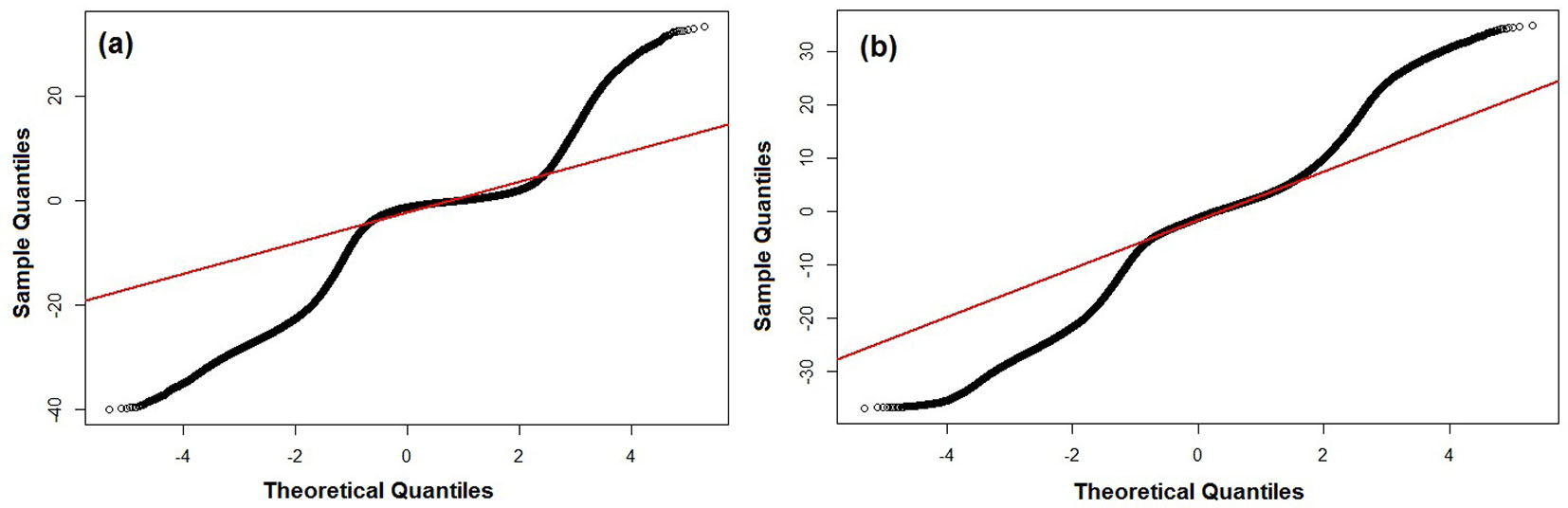
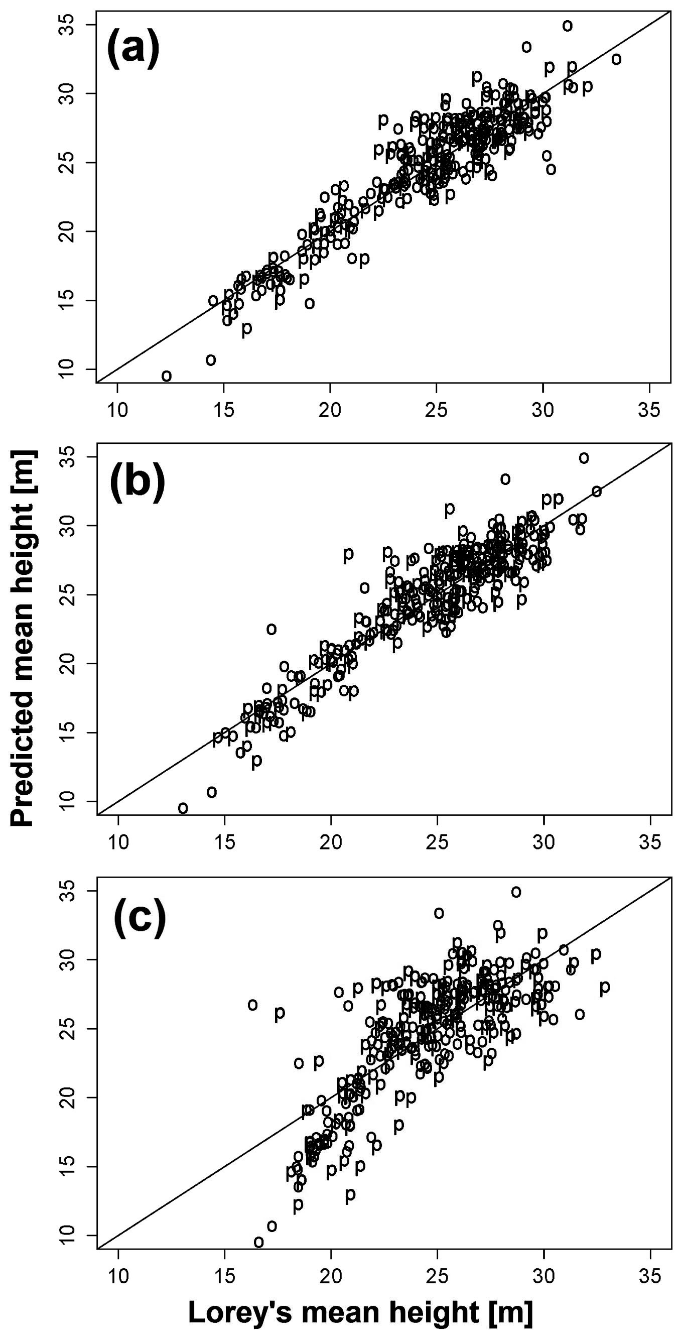
Fig. 3 - Lorey’s mean height (x-axis) plotted against the predicted mean height (y-axis). (a): CHMALS; (b): CHMSGM; and (c): CHMeATE.
We calculated the difference maps by subtracting image-based CHMs (CHMSGM and CHMeATE) of the entire study area from pure ALS (CHMALS). The difference maps were calculated only for forested areas, while all non-forested areas were excluded using forest and non-forest mask. For normality test of error distribution, we used the Q-Q plots (Fig. 2) and the Anderson-Darling’s method integrated into the “nortest” package of the R software ([8]). Since the distribution of errors was found to be non-normal (Fig. 3), we derived the accuracy assessment using sample quantiles of the error distribution based on the methodology for DEM accuracy assessment proposed by Höhle & Höhle ([14]) and Hobi & Ginzler ([11]). Using this approach, the median (50% quantile), the normalized median absolute deviation (NMAD) and the 68.3% and 95% sample quantiles were calculated from the difference maps using the R software. The NMAD was calculated according to Höhle & Höhle ([14]) as follows (eqn. 4):
where Δhj denotes the individual error (j = 1,…, n) and mΔh is the median of the errors. NMAD is thus proportional to the median of the absolute difference between errors and the median errors.
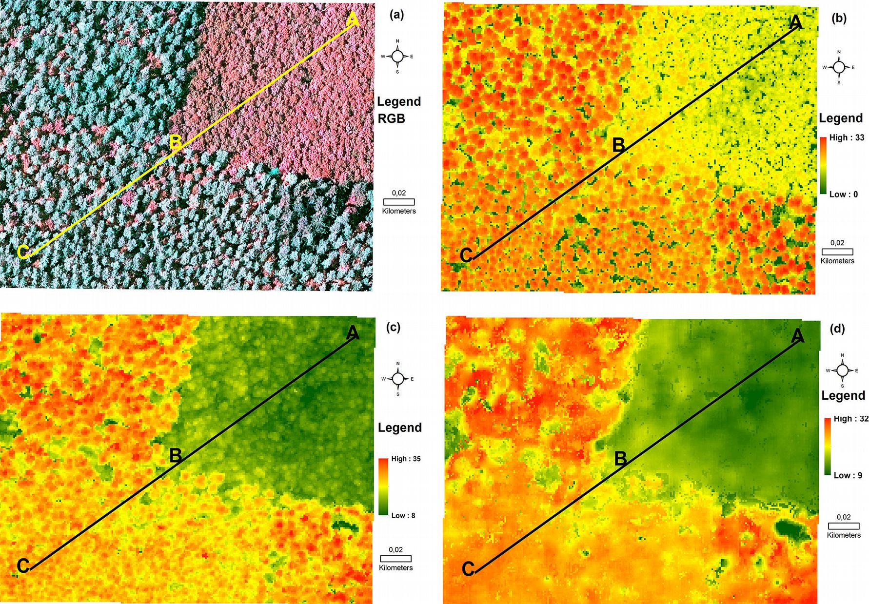
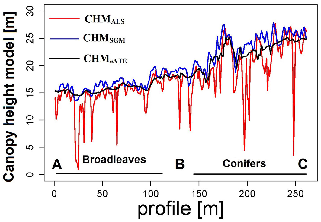
We also selected a transect line of 1.71 km as shown in Fig. 1 and Fig. 4 for visual interpretation of the trend of CHM. The height values of the CHMs falling along the transect line were extracted and plotted as line graphs (Fig. 5), in order to visually display the trend of correlation between the CHMs.
Fig. 4 - Example of the final output maps of the canopy-height models (CHM) obtained in this study, covering a small portion of the whole studied area, and including the transect line (ABC) represented in Fig. 1. (a): RGB; (b): CHMALS; (c) CHMSGM; (d) CHMeATE.
Results
Predictions of ground Lorey’s mean height (LMH)
The final most explanatory variables derived from CHMALS were the height at 99th percentile and the canopy density (cd), and we achieved R2 = 0.83 and RMSE = 1.93 m against LMH (Tab. 3). Similarly, we achieved R2 = 0.82 and RMSE = 2.09 m by using height at 95th percentiles and canopy density (cd) as explanatory variables derived from CHMSGM against LMH. However, for the CHMeATE, we achieved R2 = 0.55 and RMSE = 3.22 m by using height at 90th percentiles, standard derivation (SD) and canopy density 2 (cd2) metrics as an explanatory variables (Tab. 3).
Tab. 3 - Comparison of predicted canopy height vs. ground LMH based on 3-fold cross validation (n=296 plots). (R2): coefficients of determination; (Adj. R2): adjusted R2; (***): p < 0.001, (**): p <0.01, (*) p < 0.05, and (.): p < 0.1 indicated the level of significance after t-test.
| Canopy height model (CHM) |
Selected variables |
Coefficients | R2 | RMSE | RMSE% |
|---|---|---|---|---|---|
| CHMALS | intercept** | 4.59 | 0.83 | 1.93 | 7.92 |
| h99*** | 0.93 | ||||
| cd** | -4.45 | ||||
| CHMSGM | intercept*** | 24.46 | 0.82 | 2.09 | 8.54 |
| h95*** | 0.96 | ||||
| cd*** | -23.88 | ||||
| CHMeATE | intercept*** | 35.02 | 0.55 | 3.22 | 13.23 |
| h90*** | 0.55 | ||||
| std*** | 0.7 | ||||
| cd2*** | -24.19 |
Overall, we did not observed significant differences between the predictive power of the explanatory variables derived from CHMALS and CHMSGM for estimating LMH. However, the predictive power of explanatory variables derived from CHMeATE was not that accurate as CHMALS and CHMSGM for estimating LMH (Tab. 3).
Comparison of image-based Canopy height models (CHMSGM and CHMeATE) with pure ALS (CHMALS)
A summary of the statistics for the error distribution derived by subtracting CHMSGM, CHMeATE from CHMALS is shown in Tab. 4. We achieved a median error of -1.30 m and NMAD = 0.68 m from the difference maps derived by subtracting CHMSGM from CHMALS. However, we achieved a median error of -1.18 m and NMAD = 1.11 m from the difference map obtained by subtracting CHMeATE from CHMALS. In this case, CHMSGM was closer to CHMALS as compared to CHMeATE (Tab. 4).
Tab. 4 - Comparison of vertical agreement measures of image-based CHM (CHMSGM and CHMeATE) with pure ALS-derived CHM (CHMALS).
| Forested areas | CHMSGM - CHMALS | CHMeATE - CHMALS |
|---|---|---|
| Sample size | Summary of the statistics of the error distribution derived from the differences maps | |
| 50% (median) [m] | -1.30 | -1.18 |
| NMAD [m] | 0.68 | 1.11 |
| 68.3% | -0.57 | 0.74 |
| 95% quantile [m] | 0.99 | 6.64 |
Fig. 4 shows the final output maps of CHMs for a small subset of the study area which includes the transect line for CHMs comparison.
An example of the vertical profile of the four CHMs along the transect line depicted in Fig. 4 is shown in Fig. 5, where height values extracted from each CHMs are plotted in the form of line graphs. In general, all the three CHMs show a good agreement of the outer envelops of the forest surface. However, CHMALS seems to penetrate deeper through the small opening of the forest canopy. This suggests that image-based CHMs could be limited to the outer envelope of the forest structure and cannot describe in details both the middle layer and the forest ground.
Discussion
The first objective of our study was to compare the potential of photogrammetric image-based point clouds with ALS-derived data for the assessment of forest heights. The purpose was to find out a viable option for all those countries where stereo aerial photographs are updated on a regular basis, but ALS acquisitions are not that consistent as needed for continuous forest management. For the CHM based on ALS (CHMALS), we achieved R2 = 0.83 and RMSE = 7.92% against LMH. Similarly, we achieved R2 = 0.82 and RMSE = 8.54 % for the image-based CHM using SGM (CHMSGM) against LMH, respectively. However, we achieved R2 = 0.55 and RMSE = 13.23% for the image-based CHM using eATE (CHMeATE) with LMH, which is not that accurate as CHMALS and CHMSGM. White et al. ([47]) used SGM and compared the potential of ALS and image-based point cloud metrics for estimating LMH at the plot level. They obtained RMSE = 8.96% for ALS and 14% for image-based point clouds with LMH., i.e., a lower accuracy as compared with that obtained in this study. Järnstedt et al. ([16]) used the NGATE module of the SOCET SET for point clouds generation and compared the potential of ALS and image-based point clouds for estimating the tree mean height at the plot level. They obtained an RMSE = 18.61% for ALS and 28.23% for image-based point clouds, which is also higher than our results based on SGM. The error distribution in the form of quantiles derived from the differences maps (Tab. 4) also indicates that the image-based CHM using SGM (CHMSGM) is closer to ALS CHM (CHMALS) than the image-based point clouds using eATE (CHMeATE).
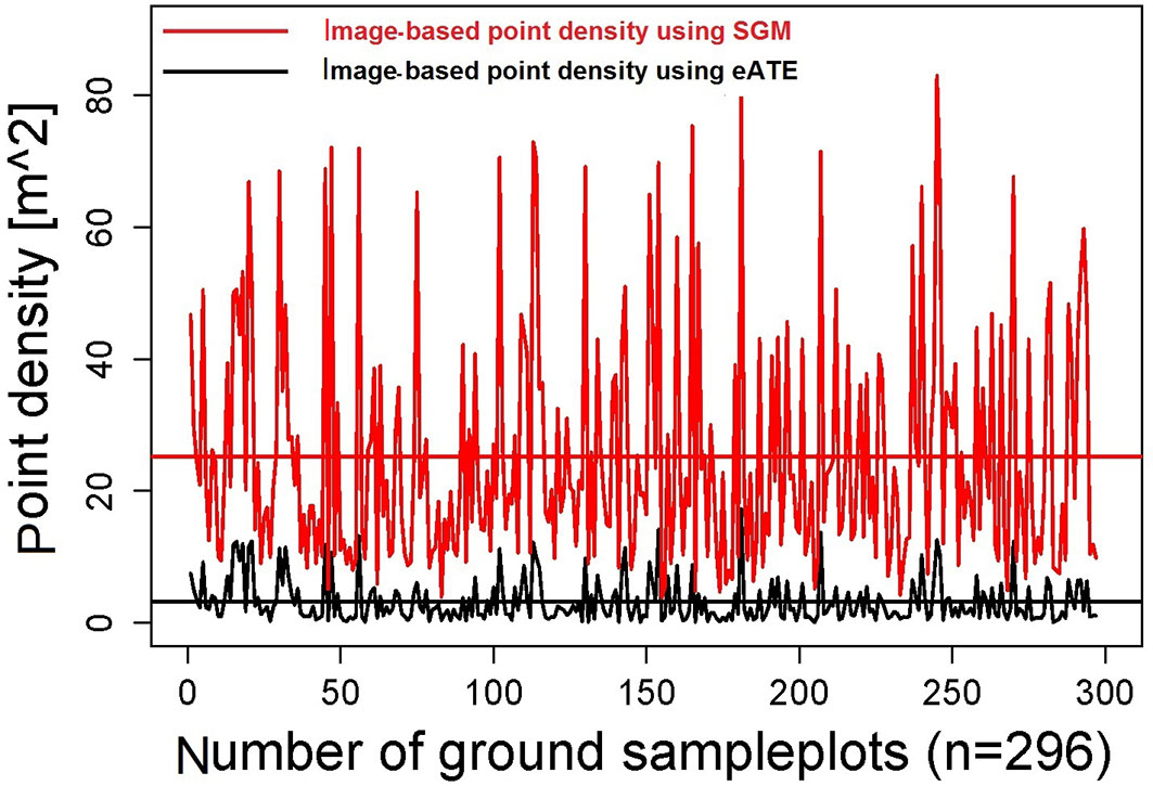
The second objective was to compare the performance of two image-matching algorithms (SGM and eATE) for estimating the canopy height. It is evident that SGM gives more accurate results than eATE by both evaluating the metrics derived from image-based CHM for predicting LMH and comparing image-based CHM (CHMSGM and CHMeATE) with ALS-derived CHM (CHMALS). We obtained reasonably accurate estimates of tree heights by using SGM image matching point clouds algorithm then eATE in combination with ALS-derived DTM. One of the reasons of the higher accuracy of SGM might be the production of point clouds. We achieved a mean point density of 25 points m-2 by using SGM and 3.19 points m-2 using eATE at sample plots location (Fig. 6). This demonstrates that point clouds based on the SGM image-matching algorithm better represent the tree structure, including the tree tops and the surrounding crown area, as compared to eATE point clouds. This difference can also be noticed from Fig. 4, where eATE-based CHM looks smoother and less coarse than SGM-based CHM. According to Gobakken & Naesset ([7]) and Magnusson ([21]), the higher is the point density, the higher will be the accuracy of forest attribute estimation. However, they compared different ALS point clouds density, while we examined first-time image-based point clouds density for determining forest heights.
Fig. 6 - Comparison of point density per square meter derived from SGM and eATE. The red graph represents mean point density [m2] derived from SGM at sample plots locations, while the straight red line represents the mean point density over all sample plots (n=296). The black line graph represents the mean point density [m2] derived from eATE at sample plots locations, while the straight black line represents the mean point density over all sample plots (n=296).
Conclusions
Our findings show that forest height information can be accurately extracted from image-based point clouds in all those forest areas where highly accurate DTMs obtained from ALS campaigns are available. The quality of such height information is comparable to ALS based product, which is a promising outcome. Further, our results confirmed that the SGM algorithm performs better than the eATE for the estimation of tree height.
ALS is the most accurate option for estimating forest structure variables and is currently used for forest management purpose in many Nordic countries. However, in many other countries, ALS data are not regularly updated as digital stereo aerial photographs, due to its high cost. So the combined approach of using image-based point clouds and historical ALS-derived DTM developed in this study offer a viable and cost-effective option to forest community for estimating height-related forest structural parameters, and can be useful for all those countries where stereo aerial photographs are updated at a regular period in the presence of pre-existing historical ALS-derived DTM.
Acknowledgments
The authors are thankful to the Shaheed Benazir Bhutto University, Sheringal Dir Upper and Higher Education Commission (HEC) of Pakistan for awarding Mr. Sami Ullah a PhD scholarship, which enabled this research work. Furthermore, we are thankful to European Commission for the financial support of the project Delivery of sustainable supply of non-food biomass to support a “resource-efficient” Bioeconomy in Europe (S2BIOM). This research work is closely linked and was partly funded by S2Biom is co-funded by the European Commission in the 7th Framework Programme (Project No. FP7-608622, Project web site: ⇒ http://www.s2biom.eu/en/). The authors are also grateful to Dr. Gerald Kändler, Forest Research Institute, Baden-Württemberg (FVA) for the provision of aerial photographs, field inventory data and related possibilities to Sami Ullah at FVA.
References
CrossRef | Gscholar
Gscholar
Gscholar
Gscholar
CrossRef | Gscholar
CrossRef | Gscholar
Online | Gscholar
Gscholar
Authors’ Info
Authors’ Affiliation
Matthias Dees
Pawan Datta
Holger Weinacker
Barbara Koch
Chair of Remote Sensing and Landscape Information System, Institute of Forest Sciences, Faculty of Environment and Natural Resources, University of Freiburg (Germany)
Forest Research Institute, Baden-Württemberg - FVA (Germany)
Corresponding author
Paper Info
Citation
Ullah S, Adler P, Dees M, Datta P, Weinacker H, Koch B (2017). Comparing image-based point clouds and airborne laser scanning data for estimating forest heights. iForest 10: 273-280. - doi: 10.3832/ifor2077-009
Academic Editor
Matteo Garbarino
Paper history
Received: Apr 06, 2016
Accepted: Oct 30, 2016
First online: Feb 23, 2017
Publication Date: Feb 28, 2017
Publication Time: 3.87 months
Copyright Information
© SISEF - The Italian Society of Silviculture and Forest Ecology 2017
Open Access
This article is distributed under the terms of the Creative Commons Attribution-Non Commercial 4.0 International (https://creativecommons.org/licenses/by-nc/4.0/), which permits unrestricted use, distribution, and reproduction in any medium, provided you give appropriate credit to the original author(s) and the source, provide a link to the Creative Commons license, and indicate if changes were made.

Web Metrics
Breakdown by View Type
Article Usage
Total Article Views: 59486
(from publication date up to now)
Breakdown by View Type
HTML Page Views: 48580
Abstract Page Views: 4388
PDF Downloads: 5262
Citation/Reference Downloads: 29
XML Downloads: 1227
Web Metrics
Days since publication: 3425
Overall contacts: 59486
Avg. contacts per week: 121.58
Article Citations
Article citations are based on data periodically collected from the Clarivate Web of Science web site
(last update: Mar 2025)
Total number of cites (since 2017): 10
Average cites per year: 1.11
Publication Metrics
by Dimensions ©
Articles citing this article
List of the papers citing this article based on CrossRef Cited-by.
Related Contents
iForest Similar Articles
Research Articles
Identification and characterization of gaps and roads in the Amazon rainforest with LiDAR data
vol. 17, pp. 229-235 (online: 03 August 2024)
Review Papers
Accuracy of determining specific parameters of the urban forest using remote sensing
vol. 12, pp. 498-510 (online: 02 December 2019)
Research Articles
Estimation of aboveground forest biomass in Galicia (NW Spain) by the combined use of LiDAR, LANDSAT ETM+ and National Forest Inventory data
vol. 10, pp. 590-596 (online: 15 May 2017)
Research Articles
Estimating biomass and carbon sequestration of plantations around industrial areas using very high resolution stereo satellite imagery
vol. 12, pp. 533-541 (online: 12 December 2019)
Research Articles
Classification of xeric scrub forest species using machine learning and optical and LiDAR drone data capture
vol. 18, pp. 357-365 (online: 07 December 2025)
Review Papers
Remote sensing-supported vegetation parameters for regional climate models: a brief review
vol. 3, pp. 98-101 (online: 15 July 2010)
Review Papers
Analysis of full-waveform LiDAR data for forestry applications: a review of investigations and methods
vol. 4, pp. 100-106 (online: 01 June 2011)
Research Articles
Integrating area-based and individual tree detection approaches for estimating tree volume in plantation inventory using aerial image and airborne laser scanning data
vol. 10, pp. 296-302 (online: 15 December 2016)
Research Articles
High resolution biomass mapping in tropical forests with LiDAR-derived Digital Models: Poás Volcano National Park (Costa Rica)
vol. 10, pp. 259-266 (online: 23 February 2017)
Research Articles
Mapping the vegetation and spatial dynamics of Sinharaja tropical rain forest incorporating NASA’s GEDI spaceborne LiDAR data and multispectral satellite images
vol. 18, pp. 45-53 (online: 01 April 2025)
iForest Database Search
Google Scholar Search
Citing Articles
Search By Author
Search By Keywords
PubMed Search
Search By Author
Search By Keyword


