High resolution biomass mapping in tropical forests with LiDAR-derived Digital Models: Poás Volcano National Park (Costa Rica)
iForest - Biogeosciences and Forestry, Volume 10, Issue 1, Pages 259-266 (2017)
doi: https://doi.org/10.3832/ifor1744-009
Published: Feb 23, 2017 - Copyright © 2017 SISEF
Research Articles
Abstract
Tropical forests play a key role in global carbon cycle. Reducing Emissions from Deforestation and forest Degradation (REDD+) program requires reliable mechanisms for Monitoring, Reporting and Verification (MRV). In this regard, new methods must be developed using updated technologies to assess carbon stocks. The combination of LiDAR technology and in situ forest networks allows the estimation of biomass with high resolution in low data environments, such as tropical countries. However, the evaluation of current LiDAR methods of biomass inventory, and the development of new methodologies to reduce uncertainty and increase accuracy, is still needed. Our aim is to evaluate new methodologies of spatially explicit LiDAR biomass inventories based on local and general plot-aggregate allometry. For this purpose, 25 field plots were inventoried, covering the structural and ecological variability of Poás Volcano National Park (Costa Rica). Important differences were detected in the estimation of aboveground biomass (92.74 t ha-1 considering the mean value of plot sample) depending on the chosen tree allometry. We validated the general aboveground biomass plot-aggregate allometry proposed by Asner & Mascaro (2014) in our study area, and we fitted two specific models for Poás forests. Both locals and general models depend on LiDAR top-of-canopy height (TCH), basal area (BA) and wood density. Small deviations in the wood density plot sample (0.60 ± 0.05) indicated that a single wood density constant value could be used throughout the study area. A BA-TCH origin forced linear model was fitted to estimate basal area, as suggested by the general methodology. Poás forest has a larger biomass density for the same THC compared to the rest of the forests previously studied, and shows that the BA-TCH relationship might have different trends in each life zone. Our results confirm that the general plot-aggregate methodology can be easily and reliably applied as aboveground biomass in a new area could be estimated by only measuring BA in field plots to obtain a local BA-TCH regression. For both local and general methods, the estimation of BA is critical. Therefore, the definition of precise basal area field measurement procedures is decisive to achieve reliable results in future studies.
Keywords
Carbon, Remote Sensing, REDD, LiDAR, Plot-level Allometry, Biomass, Basal Area
Introduction
The Fourth Assessment Report of the Intergovernmental Panel on Climate Change ([18]) reports an increment in the global average temperature related to an increase of 70% in Greenhouse Gas (GHG) emissions due to human activities since 1970 ([19]). Forests play a double role of particular importance on adjustment of the global carbon cycle, acting as both carbon emission sources and sinks. Emissions due to deforestation, degradation of the forests and land use changes encompass 17.3% of total GHG emissions ([19]). As carbon pools, the IPCC ([19]) estimates that forests contain 77% of carbon stored in global forest vegetation and 39% of carbon in soils. In this regard, tropical forests are very important as they can store more carbon per hectare than other forests ([17]), with estimates in the order of 25% of carbon in the biosphere ([8]). According to the FAO Forest Resources Assessments 2010 ([34]), the highest deforestation rates can be found in the tropics, hence tropical forests are the most threatened ecosystems on earth.
In order to curb the GHG emissions due to forest losses, Reducing Emissions from Deforestation and forest Degradation (REDD+) scheme was recognized as a valid mechanism against climate change in the 2010 Cancun Agreement (UNFCCC COP-16 Conference). Costa Rica joined this initiative integrating the carbon captured data from its National Parks and Biological Reserves into the schemes framework, which consequently became one of the main points in its REDD+ strategy approved in 2008.
A transparent system for Monitoring, Reporting and Verification (MRV) is a necessary requirement of REDD+ activity. If accurate estimates of carbon are expected then this process could prove costly; hence, it is important to develop efficient methods to carry out large-scale precise and inexpensive measurements. Wall-to-wall high resolution estimations of biomass and carbon stocks in tropical areas are crucial to quantify emissions from forest loss, gain and growth, but also to identify, describe, and quantify emissions from forest degradation. Quantifying emissions from forest degradation in tropical forests is a major concern as forest degradation might represent a significant percentage of nationwide emissions of greenhouse gases ([27]). Some authors pointed out that those emissions from forest degradation can be of the same magnitude as those caused by deforestation ([32]). Wall-to-wall mapping can lead to a better understanding of land use dynamics and an easier identification of drivers of forest degradation and deforestation. Therefore, the incorporation of these methods could lead to a substantial improvement in forest management, supporting the formulation of environmental policies, planning tools and actions to improve the status and conservation of forests.
Light Detection and Ranging (LiDAR) is an active remote sensing technique based on a laser sensor. It is a powerful technology for accurate estimates of the spatial variability in forest carbon stocks. Although LiDAR data acquisition may be expensive ([15], [29]), it is the most appropriate technology at scales ranging from one to several million hectares and is useful for calibrating broader-scale Interferometric Synthetic Aperture Radar measurements ([33]). Other authors ([25]) showed that space-based LiDAR, such as the Geoscience Laser Altimeter System, might be useful as a resource to assist the mapping of forest biomass carbon stocks using the classification of high resolution optical rather than radar data.
The effectiveness of LiDAR technology to estimate forest variables in tropical forest has been proved in different works. Clark et al. ([11]) estimated mean tree height for plantation plots at La Selva Biological Station (Costa Rica) using plot mean LiDAR height with a model R2 of 0.97 and 1.08 m of root-mean-square error (RMSE). Clark et al. ([12]), also working in La Selva forest, obtained an aboveground biomass model with an R2 of 0.90 and RMSE of 38.3 Mg ha-1 including in the model two LiDAR metrics (plot-level mean height and maximum height).
Asner et al. ([3]) used the vertical center of canopy volumetric profile, also known as mean canopy profile height (MCH) to fit regional and universal models. These authors were able to predict aboveground carbon density in different tropical locations using a single universal LiDAR model (R2 = 0.80, RMSE = 27.6 Mg C ha-1). Although this approach showed to be consistent when using a single LiDAR sensor ([3]), an approach based on the variable top-of-canopy height (TCH) has proved to be more consistent across different sensor characteristics ([6]). Therefore, the latter authors developed a general plot-aggregate allometry based on the TCH variable using a LiDAR plot network of tropical forest sites in Colombia, Hawaii, Madagascar, Peru and Panama to evaluate carbon density across a wide range of tropical vegetation conditions. TCH is derived from the LiDAR digital canopy model and is a consistent index among different modern LiDAR sensors ([6]). According to them, this general methodology can largely reduce fieldwork for LiDAR inventories in tropical areas because aboveground biomass could be estimated by only measuring basal area in field plots to obtain regional basal area-TCH regression.
The aim of this paper is to validate the general aboveground biomass (AGB) plot-aggregate equation developed by Asner & Mascaro ([6]) in Poás forest (Costa Rica) and to compare the results found through this model to those obtained through local models fitted for the study area. The main objective was to assess the validity of this general model and the advantages of fitting local models instead of using the Asner & Mascaro’s equations. Poás Volcano National Park is an appropriate area to test this AGB plot-aggregate approach due to the large structural and ecological variability in the area. Furthermore, to evaluate the importance of the tree allometry in wall-to-wall AGB estimations, two general individual tree allometric biomass equations proposed by Chave et al. ([9]) have been used.
Material and methods
Study area and input data
The study was carried out in the Poás Volcano National Park (6506 ha), in the province of Alajuela (Costa Rica - Fig. 1). It is a stratovolcano complex with a generally steep terrain ranging from 1099 to 2713 m in elevation, with a mean annual precipitation and temperature gradient of approximately 2300-5100 mm y-1 and 9-15 oC, respectively. Due to the existence of two slopes (Atlantic and Pacific slopes), an abrupt topography and a wide altitude range is observed, with significant fluctuations in mean annual precipitation and temperature throughout the study area.
Fig. 1 - Location of Poás Volcano National Park in Alajuela Province (Costa Rica) and spatial distribution of field plots and Holdrige’s life zones in the area.
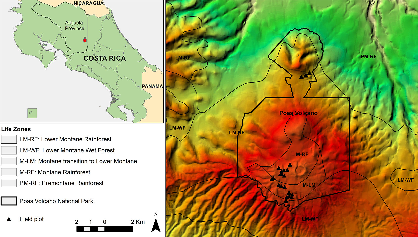
According to the ecological map of Costa Rica ([7]). Poás Volcano area hosts forests corresponding to Holdridge’s life zones of montane rainforest (M-RF), lower montane rainforest (LM-RF), montane transition to lower montane rainforest (M-LM), premontane rainforest (PM-RF) and lower montane wet forest (LM-WF - Fig. 1).
Input data was a 1-m resolution Digital Elevation Model (DEM) and a Digital Surface Model (DSM) generated from an airborne LiDAR flight executed by Stereocarto S.L. in July 2010. The area was surveyed with the ALS50-II-MpiA sensor (multi pulse in air) achieving a mean point density of 1 point m-2. These data were projected in the CR05 Reference System and the Transversal Mercator projection for Costa Rica CRTM05. A Digital Canopy Model (DCM) that represents the maximum vegetation height in each 1-m pixel was obtained from the subtraction of the DEM and the DSM.
In order to encompass the range of structural and ecological variability in the Park, a stratified sample throughout the different life zones of Holdridge was conducted. For this, we generated LiDAR-derived canopy height maps to identify the vertical and horizontal structural differences in the forest. Thus, a 20 m resolution raster was built from a three statistics code. The three parameters measured in each 20×20 pixel were: (i) canopy cover as percentage of 0×1 m pixels above 2.00 m; (ii) 95th height percentile (P95); and (iii) interquartile range (IQ). They were codified in class values taking into account each parameter range (Tab. 1)
Tab. 1 - Parameters measured in each 20×20 pixel to generate a code characterizing the vegetation structure of Poás National Park (Costa Rica).
| Variable | Range | Value |
|---|---|---|
| Canopy cover | 0-85.5 % | 1 |
| 85.5-99.5 % | 2 | |
| 99.5-100 % | 3 | |
| P95 | 2-21 m | 1 |
| 21-27 m | 2 | |
| >27 m | 3 | |
| IQ | 0-5 m | 1 |
| 5-8 m | 2 | |
| >8 m | 3 |
Field lot estimation
Transects were designed following the roads and trails within the study area and a total of 25 circular sampling plots of 0.04 ha were established encompassing the structural variability of the area through the generated code (Tab. 1). Thus, LiDAR information was used in the sampling design process generating field sample plots which included the highest percentage of structural variability in the domain.
All plot locations were maintained at a proper distance from the roads and trails to avoid their possible effect (Fig. 1). In each 0.04 ha plot, we measured and identified all woody stems with diameter at breast height (DBH) ≥ 5 cm until the highest possible taxonomic level. The heights of all ferns and palms were measured with hypsometer Vertex III. All plots were located with a GPS Garmin GPSmap76Cx using the CRTM05 projection. This GPS device provides a typical Differential Global Positioning System horizontal accuracy lower than 5 meters.
Tab. 2 - Tree allometric equations used for aboveground biomass estimates in Poás Volcano National Park (Costa Rica). (nd): not determined.
| Equation | DBH range (cm) |
Number of individuals |
R2 |
|---|---|---|---|
| Chave et al. (model I) | ≥5 - 133.2 | 419 | nd |
| Chave et al. (model II) | ≥5 - 133.2 | 419 | nd |
| Frangi & Lugo | - | 25 | 0.96 |
| Tiepolo et al. | - | 22 | 0.88 |
Aboveground biomass for each tree (agb) inventoried in the plots was estimated using two different allometric models (Tab. 2). We used and compared the tropical wet forest stands allometric equations provided by Chave et al. ([9]). In particular, model I was expressed as follows (eqn. 1):
while model II had the following form (eqn. 2):
where agb is the estimated individual tree oven-dry aboveground biomass (kg), DBH is the tree stem diameter at 1.3m (cm), h is the tree height (m) and ρ is the wood specific gravity (oven-dry wood over green volume, g cm-3).
Measuring tree height is a hard task in this type of forest, so we used a combination of LiDAR measurements and diameter-based estimation to develop a height-diameter model. The maximum LiDAR height was related through a power regression with the maximum field measured diameter in each sample plot, in order to avoid unrealistic tree height estimates ([5]). This regression was applied to estimate each tree height.
Palms biomass was estimated using the equation (eqn. 3) proposed by Frangi & Lugo ([14]) for the moist forests of Puerto Rico of Prestoea montana (Graham) G. Nicholson. The equation (eqn. 4) proposed by Tiepolo et al. ([36]) for the Cyathea genus of tropical montane moist forests of Serra do Mar National Park, Brazil was used to estimate a ferns biomass (eqn. 3, eqn. 4):
where agb is the estimated oven-dry aboveground biomass (kg) and h is the height (m) in both equations.
To estimate each tree wood specific gravity, we followed the Global Wood Density Database ([10], [38]). When it was not possible to use a value for a particular species, an average value at genus or family level was used. The 2008 Readiness Preparation Proposal ([24]) average values of wood density were applied when it was not possible to assign species, genus or family to the measured trees. These values are based on the research of Chudnoff cit. Solórzano ([35]).
Aboveground biomass (AGB) of each field plot is the sum of the oven-dry aboveground biomass of all individual trees (agb), palms and ferns in the plot, expressed per hectare (Tab. 3).
Tab. 3 - Summary of the field plot parameters (n = 25) for aboveground biomass modeling in Poás Volcano National Park (Costa Rica). AGB has been calculated using two different tree-allometric equations from Chave et al. ([9])
| Parameters | Mean | Minimum | Maximum | Standard Deviation |
|---|---|---|---|---|
| BA (m2 ha-1) | 58.50 | 30.97 | 84.11 | 13.04 |
| Wood density (g cm-3) | 0.60 | 0.51 | 0.70 | 0.05 |
| Stem number (stems ha-1) | 1699.00 | 425.00 | 2500.00 | 546.94 |
| TCH (m) | 15.28 | 8.51 | 20.74 | 3.34 |
| AGB Chave’s model I (t ha-1) | 312.42 | 133.76 | 580.32 | 104.62 |
| AGB Chave’s model II (t ha-1) | 405.16 | 168.26 | 987.69 | 175.10 |
Plot-aggregate allometry
We calculated for each sample plot the top-of-canopy height (TCH) ([6]) which is considered as the average height of all 1 m resolution pixels of the Digital Canopy Model inside sample plots.
Tropical tree crowns can reach over 20 m in diameter; therefore, large probabilities exist for tree crowns to overlap adjacent 20×20 m plots. This limitation of the available field data may affect the results of the survey, so we increased cell size for processing LIDAR data to 25×25 m. In addition, by increasing cell size it is possible to minimize errors due to low GPS location accuracy, thus improving overlap between DCM cells and sample plots and ensuring that measured trees are taken into account in the remote sensing analysis.
Asner et al. ([2]) proposed a plot-aggregate allometry inspired by the general tree allometric theory of Chave et al. ([9]), which assumes that biomass follows the equation (eqn. 5):
where agb is individual tree aboveground biomass, DBH is stem diameter (cm), h is canopy height (m), ρ is wood specific gravity (wood density, g cm-3) and a, b1, b2 and b3 are the model parameters.
On the basis of this model, Asner & Mascaro ([6]) fitted a general model of plot-aggregate aboveground biomass using a LiDAR plot network of tropical forest sites in Colombia, Hawaii, Madagascar, Peru and Panama to evaluate carbon density across a wide range of tropical vegetation conditions (eqn. 6):
where AGB is the total plot aboveground biomass (t ha-1), TCH is LiDAR-derived top-of-canopy height (m), BA is plot-averaged basal area (m2 ha-1) and ρBA is basal-area weighted wood density (g cm-3). The general model was originally fitted to estimate aboveground carbon density. A factor of 0.48-1 ([21]) was used to convert aboveground carbon density model into aboveground biomass.
This method reduces the need for exhaustive plot-based inventories ([6]) by relating TCH with BA, and TCH with wood density at regional level. Thus, BA is the only variable to be measured during the inventory, since density is considered as an average constant value for the plot.
We validated the general Asner & Mascaro’s plot-aggregate allometry equation in our study area and we also fitted two specific models for the Poás Volcano forest following the same structure, one model using AGB estimations from Chave’s equations I and the other one using AGB estimations from Chave’s equation II. In order to fit the power AGB models we used the Nonlinear Least Squares (nls) function from the “stats” package included in the R software ([30]). This function determines the nonlinear (weighted) least-squares estimate of the parameters of a nonlinear model using a Gauss-Newton algorithm.
Asner & Mascaro ([6]) proposed a simple linear model forced through the origin to capture the BA variation in each region. This BA-TCH origin forced regression assumes that with a TCH of zero, BA must not be greater than zero. This ratio between BA and TCH is called a stocking coefficient (SC - [4]) and explains structural variability across different tropical forests. In our study area, SC was estimated using a similar origin forced linear model.
Bias (b), root mean squared error (RMSE), relative bias (b%) and relative mean squared error (RMSE%) were calculated as principal contrasting statistics in the fitting phase of the AGB local model and in the validation of the general model in our study area (eqn. 7, eqn. 8, eqn. 9, eqn. 10):
where AGBi is the true or reference aboveground biomass measured in field plots, AGÌÂBi is the aboveground biomass estimated by the model, n is the number of plots and AGB is the mean of the AGB field plot sample.
We mapped AGB across the landscape with LiDAR metrics using resolution of 25× 25 m, i.e., each grid cell had the same area as cells used for LiDAR metrics processing, as other authors have already indicated ([20]). Top-of-canopy height, basal area and basal area weighted wood density were estimated in each cell. We then applied to each grid cell the general model and the two Poás forest models specifically fitted for this area.
Results and discussion
Field measured biomass
AGB for each plot was calculated using two different Chave’s equations (eqn. 1 and eqn. 2). In order to use eqn. 1, single tree heights obtained through the height-diameter model were computed (eqn. 11)
(R2 = 0.49, RMSE = 3.97 m - see Fig. S1 in Supplementary material) where h is total tree height (m) and DBH is stem diameter (cm).
Aboveground biomass values (average ± standard deviation) estimated from the 25 field plots were 312.42 ± 104.62 t ha-1 when Chave’s model I (eqn. 1) was used and 405.16 ± 175.1 with Chave’s model II (eqn. 2). Mean basal area resulted in a value of 58.50 ± 13.04 m2 ha-1 and average estimated wood density was 0.60 ± 0.05 g cm-3 (Tab. 3).
We observed important differences in the estimation of AGB (92.74 t ha-1 considering the mean value of plot sample) depending on the chosen tree allometry, affecting considerably and systematically the continuous estimation of AGB in the study area. Measuring heights of several dominant and intermediate trees with hypsometer in the plots could have improved this regression curve, though this option was not feasible during fieldwork due to time and budget constraints. Allometric errors, including systematic errors derived from the height-diameter model, might be the main cause of the differences when Chave’s I and Chave’s II models are used in the study area. Other authors have fixed the maximum LiDAR height to the maximum measured diameter for the same field plot to obtain a height-diameter model. This was considered as a conservative method to constrain their field-estimated carbon stocks for tropical dry forests and mangroves in Panama ([5]).
Plot-aggregate allometry
Basal area was related to TCH through the origin forced linear regression BA-TCH (Tab. 4). Both variables show significant correlation (p-value < 0.001). The stocking coefficient in our sampling (SC = 3.70) is higher than those reported by Asner & Mascaro ([6]) in other tropical areas (1.13-2.58). This situation shows that Poás forest has larger biomass density for the same THC than the rest of the forests studied by Asner & Mascaro ([6]).
Tab. 4 - Stocking coefficient (SC), local and general AGB models used in the study area. The parameters for the general model are taken from Asner & Mascaro ([6]), while parameters for the local models have been adjusted for this work.
| Models | Units | a | b1 | b2 | b3 | SC | RMSE |
|---|---|---|---|---|---|---|---|
| Local basal area model | m2 ha-1 | - | - | - | - | 3.7 | 15.62 |
| General model (Asner&Mascaro) | t ha-1 | 7.9912 | 0.2807 | 0.9721 | 1.3763 | - | 34.26 |
| Local model (Chave’s model I) | t ha-1 | 1.82137 | 0.3299 | 1.17488 | 1.05626 | - | 30.33 |
| Local model (Chave’s model II) | t ha-1 | 1.92262 | 0.30201 | 1.17260 | 0.59760 | - | 32.80 |
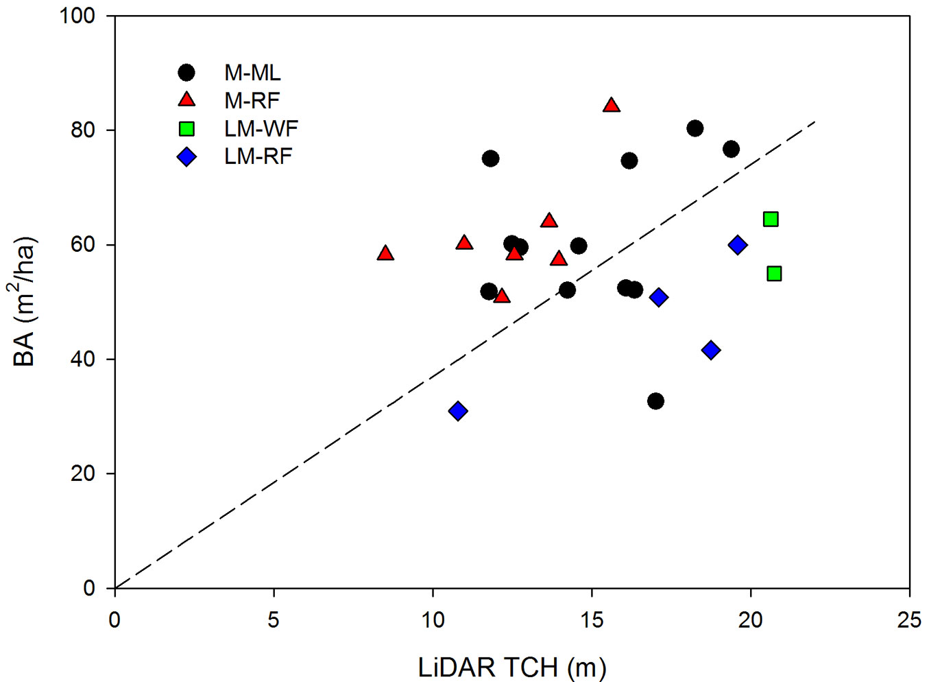
Asner & Mascaro ([6]) suggests that the SC varies regionally, e.g., Asner et al. ([5]) used only one AGB-TCH model to estimate aboveground biomass throughout the Republic of Panama. Although in this work SC was estimated for the entire area, the results show that SC might have different trends in each life zone (Fig. 2). The low number of plots constrained the estimation of reliable SC for different Holdridge’s life zones.
Fig. 2 - Relationship between LiDAR top of canopy heights (TCH) and basal area (stocking coefficient, SC) in each Holdridge’s life zone of the Poás Volcano National Park (Costa Rica).
Through the general model, aboveground biomass was estimated using only the field BA measurements. Asner & Mascaro ([6]) suggested that relascope methods may be appropriate for quick BA measurements in-field. However, this method requires the development of a methodology to estimate a reliable TCH in variable-radius inventories.
There was no significant correlation between basal area weighted wood density and TCH (R2 = 0.0014 and p-value > 0.05). These results combined with the small deviation of basal area weighted wood density in sampling (0.60 ± 0.05) suggest that it is possible to use a wood density constant value for the entire study area.
In the fitting phase the local models obtained a RMSE of 30.33 t ha-1 and 32.80 t ha-1 and were generated following the same structure as the general model (Tab. 4). The independent variables were significant at the 0.05 level. However, the models were not as consistent as before when basal area estimations from TCH were incorporated in the local model (Fig. S2 in the Supplementary material). This indicates low fitting of TCH and BA in this area and therefore, larger plots and/or different fits per life zone are required.
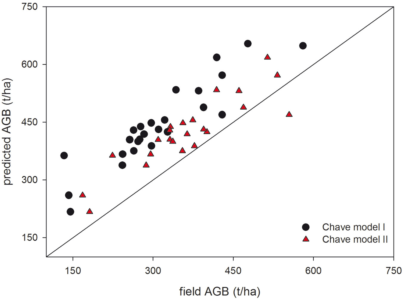
The comparison of AGB field plots measurements using Chave’s model I and Chave’s model II with AGB estimations obtained using the general model by Asner & Mascaro ([6] - Tab. 5) shows a better performance when Chave’s II is used (Fig. 3), even though both models produce systematic deviations.
Tab. 5 - Comparison of the results obtained by the Asner & Mascaro’s general model with the Chave’s model I and model II and field measured basal area value (FM) or the stocking coefficient basal area value (SC). b is the bias, RMSE is the root mean squared error, b% is the relative bias and RMSE% is the relative mean squared error.
| agb model | BA | b | RMSE | b% | RMSE% |
|---|---|---|---|---|---|
| Chave’s model I | FM | -130.56 | 137.29 | -41.79 | 43.94 |
| Chave’s model I | SC | -120.24 | 166.83 | -38.49 | 53.40 |
| Chave’s model II | FM | -37.82 | 102.27 | -9.33 | 25.24 |
| Chave’s model II | SC | -27.50 | 164.62 | -6.79 | 40.63 |
Fig. 3 - Estimated values of aboveground biomass using LiDAR derived data and the general approach ([6]) against estimated aboveground values using field measurements and tree allometric equations of Chave’s model I and model II in Poás Volcano National Park (Costa Rica).
The general model was validated by the field plots measured data (BA and BA-weighted wood density) and by the estimated variables (predicted BA from SC and predicted mean weighted wood density - Tab. 5). Using Chave’s equation II, the general model had low bias when SC was applied (b = -27.5 t ha-1, b% = -6.79%). The large RMSE in the general model validation (more than 100 t-1) was likely due to the small size plot. Small size plot generates large errors due to field sampling errors ([31]). In addition, small size plot increase the influence of edge effect and GPS errors in TCH and AGB field plot measurements. Mauya et al. ([22]), working with AGB plot-level LiDAR models in northern Tanzania, reported that relative root mean square error decreased from 63.6 to 29.2% when the size plot was increased from 0.02 to 0.3 ha. We obtained a relative RMSE similar to that of Mauya et al. ([22]) for similar plot size (0.04 ha).
Differences between field plots size and cell size for processing LiDAR data can be considered as an error source. Working with a large scale global data set, Réjou-Méchain et al. ([31]) simulated the field sampling errors derived from the utilization of different sizes in field plots and remote sensing footprint. They showed that when field plots were very small (0.1 ha and below), the sampling error was mostly due to the contribution from field sampling, and was relatively insensitive to footprint area. According to that, we expect that AGB errors in Poás forest are more likely influenced by the small size of field plots than by the differences between the field plots size and the cell size for processing LiDAR data.
Our plot size (0.04 ha) was smaller than the one used for generating the general model (0.1-1.0 ha). Using small plots for estimating AGB or BA may result in improper estimations ([23], [22]). Optimizing plot size is likely to be dependent not on plot size per se, but on the ratio of typical crown sizes to the plot size ([6]). Three important outcomes are achieved using larger plots (> 0.5 ha): (1) the accuracy of plot-level biomass allometry improves as the number of trees increases ([6]); (2) larger plots minimize the negative effect produced by low location accuracy due to GPS; (3) as tree crowns can exceed 20 m in diameter, it is possible that a tree crown studied in LiDAR data may not be part of a tree within the sample plot, leading to the so-called “edge effect”. These three effects could be minimized by increasing plot size ([23]), though leading to higher inventory costs. Additionally, size plots close to 1 ha could also be appropriate, as recent studies in tropical forests demonstrated that uncertainties approach 10% when plot sizes increase up to 1 ha ([6], [39]).
Plot-aggregate AGB models have biological meaning since main biomass factors are involved, i.e., height, diameter (through basal area) and wood gravity. Height and diameter determine the tri-dimensional structure of forests and wood gravity details the stored carbon per unit volume.
In these types of forests large tree crowns in overstorey layers leads to an increase of first returns from the upper level of canopy recorded by the LiDAR system, overlooking the lower strata ([13]). In this respect, TCH has broadly proved to be a good predictor of forest structure, carbon density and biomass in tropical vegetation ([6]).
Mapping biomass
Basal area values for the entire National Park were derived from the origin forced linear regression BA-TCH (Fig. 4). We used three AGB models (the general model and the two local fitted models) in order to map the AGB throughout the Holdridge’s life zones in the study area (Fig. 5). We did not take into account cells with TCH under 4.5 m for a real comparison of stored biomass in each Holdridge’s life zone, because of the extension of bare and shrub land, especially in the vicinity of crater areas and the bare eroded areas by lava streams.
Fig. 4 - Top-of-canopy Height (TCH) and Basal Area (BA) values for Poás Volcano National Park (Costa Rica). TCH values were obtained through LiDAR data and BA values were derived from an origin-forced linear regression BA-TCH.
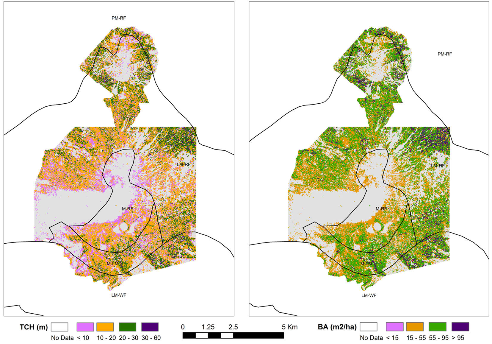
Fig. 5 - Distribution of estimated AGB (t ha-1) in the study area of Poás Volcano National Park (Costa Rica). AGB was estimated by: (a) the general model ([6] ); (b) the local model using Chave’s model I; and (c) the local model using Chave’s model II.
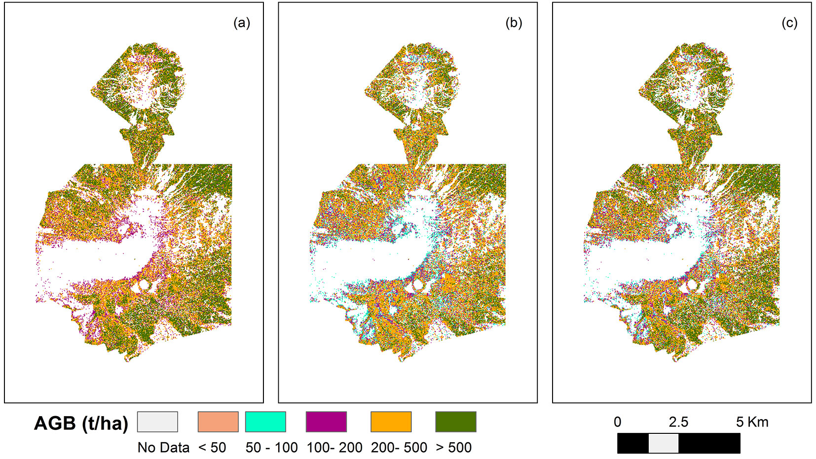
The implementation of both locals and general models resulted in consistent and logical maps that showed no big differences between neighbor cells and yielded biomass values within the expected range for this type of forests (Fig. 5). The important differences observed in the estimation of AGB depending on the chosen tree allometry affects systematically to AGB mapping in the study area (Fig. 5). The total amount of AGB for the study area is considerably larger in the case of using local model I or the general model than using local model II. This points out the importance of individual tree biomass allometry in wall-to-wall aboveground biomass mapping.
Some authors have indicated the importance of the equivalence between the size of field plots and the size of pixel LiDAR processing ([20]). We have utilized the same size for the TCH computation in the field plots and in the whole area (25×25 m). This size is slightly smaller than the 30×30 m resolution used by Clark et al. ([12]) or the 33×33 m used by Asner et al. ([1]), simulating a typical biomass sample plot used in many tropical forests studies ([28]).
Average values of 461.54 t ha-1, 409.35 t ha-1 and 336.08 t ha-1of AGB were determined for forest areas of Poás Volcano when general model, local model II and local model I were used, respectively. There are significant differences in total AGB in the study area depending on the applied model. The general model provided higher AGB than the local models, 11% higher than using local model II and 27% higher than local model I. Tree allometry is the main factor to explain these differences. Asner & Mascaro ([6]) prioritized tree-level allometries based on local information, and measured tree height at least for the three largest trees in each plot, estimating the remaining tree heights using height-diameter allometry at the species or regional level. The general model was elaborated using a more adequate local tree allometry to each particular case, instead of the one used in this work. Therefore, the results derived from the general model are more likely adjusted to reality. The elaboration of local allometry models is an expensive process; thus, the general model is an adequate alternative when LiDAR data but not local tree-allometry are available in a specific area.
In all cases, the highest mean AGB value among life zones corresponded to premontane wet forest, situated at lower altitude, while the lowest value was achieved in the highest areas, i.e., montane wet forest (Fig. 5). Thus, there is a biomass gradient with greater carbon stored in premontane wet forests, which are found at lower elevations where there is the highest rainfall (> 4000 mm y-1) and located in the Pacific side of the Park (Fig. 5). This gradient has in the same trend reported by other tropical biomass studies ([16], [37], [26]).
Conclusions
Allometry equations for the estimation of individual tree biomass are a critical factor to ensure wall-to-wall unbiased and accurate aboveground biomass mapping when plot-aggregate AGB local models are to be developed in new areas. AGB estimation can vary considerably depending on the tree allometric equations chosen or adjusted for a given study area. Differences between the results obtained with the general and the local models in our study area were significantly influenced by the applied tree allometry. The construction a local-specific allometry could improve the results, but it is more expensive. Therefore, a cost-benefit analysis might be carried out.
The alternative to developing specific tree allometry and local plot-aggregate models is the general plot-aggregate methodology, which can be easily and reliably applied. Aboveground biomass in a new study area could be estimated by measuring only the basal area (BA) in field plots in order to obtain a local BA-TCH regression. It presents an advantage over traditional intensive inventories for mapping biomass and carbon density in tropical forests, since local tree allometry and expensive time-consuming inventories are no longer required. It shows an easier approach to obtain BA through LiDAR top-of-canopy height (TCH) data, since BA is the only field measurement required. Therefore, the definition of precise BA field measurement procedures (e.g., location, size and shape of the field plots) is decisive to achieve reliable results in future studies. We confirmed the influence of plot size on BA-TCH fittings; hence, an increment of plot size is recommended for future studies.
The results of this study show that the stocking coefficient (SC) may vary locally, even in small geographical areas (few thousand ha as the study area). More fieldwork is needed to demonstrate how SC varies between different life zones. The Poás Volcano National Park showed high values of SC, which implied that its forests exhibit a larger biomass density for the same THC compared to the rest of the forests studied by Asner & Mascaro ([6]). Average basal area (58.50 ± 13.04 m2 ha-1) in the Poás Volcano National Park is significantly higher than in other forests. This parameter has a major influence on biomass storage, suggesting that these forests might play an important role as carbon sinks. In this sense, their protection and conservation is essential in a country devoted to a carbon neutral goal.
Acknowledgements
This work received a travel grant from the Technical University of Madrid. Poás Volcano National Park provided assistance, transport and lodging for the fieldworks. Authors thank Dr. Javier Bonatti (University of Costa Rica) for support, data access and sharing instruments for fieldwork.
References
CrossRef | Gscholar
CrossRef | Gscholar
Gscholar
CrossRef | Gscholar
CrossRef | Gscholar
Gscholar
Gscholar
CrossRef | Gscholar
Gscholar
CrossRef | Gscholar
Gscholar
Gscholar
Gscholar
Gscholar
Authors’ Info
Authors’ Affiliation
José Antonio Navarro
Nur Algeet-Abarquero
Agresta Soc. Coop, C/ Duque de Fernán Núñez 2, Madrid 28012 (Spain)
Sonia Condés
Dept. Natural Systems and Resources, Technical University of Madrid. School of Forestry, Ciudad Universitaria, Madrid 28040 (Spain)
Miguel Marchamalo
Dept. of Land Morphology and Engineering, Technical University of Madrid, Ciudad Universitaria, Madrid 28040 (Spain)
Corresponding author
Paper Info
Citation
Fernández-Landa A, Navarro JA, Condés S, Algeet-Abarquero N, Marchamalo M (2017). High resolution biomass mapping in tropical forests with LiDAR-derived Digital Models: Poás Volcano National Park (Costa Rica). iForest 10: 259-266. - doi: 10.3832/ifor1744-009
Academic Editor
Davide Travaglini
Paper history
Received: Jun 18, 2015
Accepted: Oct 20, 2016
First online: Feb 23, 2017
Publication Date: Feb 28, 2017
Publication Time: 4.20 months
Copyright Information
© SISEF - The Italian Society of Silviculture and Forest Ecology 2017
Open Access
This article is distributed under the terms of the Creative Commons Attribution-Non Commercial 4.0 International (https://creativecommons.org/licenses/by-nc/4.0/), which permits unrestricted use, distribution, and reproduction in any medium, provided you give appropriate credit to the original author(s) and the source, provide a link to the Creative Commons license, and indicate if changes were made.

Web Metrics
Breakdown by View Type
Article Usage
Total Article Views: 54643
(from publication date up to now)
Breakdown by View Type
HTML Page Views: 44563
Abstract Page Views: 4657
PDF Downloads: 3978
Citation/Reference Downloads: 27
XML Downloads: 1418
Web Metrics
Days since publication: 3410
Overall contacts: 54643
Avg. contacts per week: 112.17
Article Citations
Article citations are based on data periodically collected from the Clarivate Web of Science web site
(last update: Mar 2025)
Total number of cites (since 2017): 3
Average cites per year: 0.33
Publication Metrics
by Dimensions ©
Articles citing this article
List of the papers citing this article based on CrossRef Cited-by.
Related Contents
iForest Similar Articles
Review Papers
Remote sensing-supported vegetation parameters for regional climate models: a brief review
vol. 3, pp. 98-101 (online: 15 July 2010)
Review Papers
Accuracy of determining specific parameters of the urban forest using remote sensing
vol. 12, pp. 498-510 (online: 02 December 2019)
Review Papers
Remote sensing of selective logging in tropical forests: current state and future directions
vol. 13, pp. 286-300 (online: 10 July 2020)
Research Articles
Estimation of aboveground forest biomass in Galicia (NW Spain) by the combined use of LiDAR, LANDSAT ETM+ and National Forest Inventory data
vol. 10, pp. 590-596 (online: 15 May 2017)
Technical Reports
Detecting tree water deficit by very low altitude remote sensing
vol. 10, pp. 215-219 (online: 11 February 2017)
Review Papers
Analysis of full-waveform LiDAR data for forestry applications: a review of investigations and methods
vol. 4, pp. 100-106 (online: 01 June 2011)
Research Articles
Identification and characterization of gaps and roads in the Amazon rainforest with LiDAR data
vol. 17, pp. 229-235 (online: 03 August 2024)
Research Articles
Geostatistical techniques for estimating aboveground biomass in eastern Amazonia
vol. 19, pp. 85-93 (online: 13 March 2026)
Research Articles
Classification of xeric scrub forest species using machine learning and optical and LiDAR drone data capture
vol. 18, pp. 357-365 (online: 07 December 2025)
Research Articles
Mapping the vegetation and spatial dynamics of Sinharaja tropical rain forest incorporating NASA’s GEDI spaceborne LiDAR data and multispectral satellite images
vol. 18, pp. 45-53 (online: 01 April 2025)
iForest Database Search
Search By Author
Search By Keyword
Google Scholar Search
Citing Articles
Search By Author
Search By Keywords
PubMed Search
Search By Author
Search By Keyword


