Quantitative simulation of C budgets in a forest in Heilongjiang province, China
iForest - Biogeosciences and Forestry, Volume 10, Issue 1, Pages 128-135 (2016)
doi: https://doi.org/10.3832/ifor1918-009
Published: Nov 06, 2016 - Copyright © 2016 SISEF
Research Articles
Abstract
Recently, forest carbon (C) budgets have been significantly affected by climate variability, nitrogen (N) deposition, an increasing global atmospheric CO2 concentration, and disturbances (i.e., harvests, fires, and insect infestations). In this study, we quantitatively simulated the annual carbon balance of forests in Heilongjiang, China, from 1901 to 2013 using the Integrated Terrestrial Ecosystem Carbon (InTEC) model, which integrated the effects of nondisturbance (i.e., atmospheric CO2 concentration, N deposition, and climate variability) and disturbance factors. The average net primary production (NPP) of Heilongjiang was 284 g C m-2 a-1 in 1901 and increased in 1950 to 339 g C m-2 a-1; a rapid increase occurred after 1980, with an increase of 48% in 2013 compared with the NPP in 1901. The average NPP of the entire Heilongjiang region increased significantly and became more stable in 2013. However, the NPP in the northern region of the Xiaoxing’an Mountains was lower than that in the other regions. The fluctuation in average net ecosystem production (NEP) was relatively large because Heilongjiang was a carbon source for many years before the 1930s and again in the early 21st century, due to serious disturbances and intensified human activities. In recent years, NEP began to increase again, and in 2013 the forests became a large carbon sink (188 g C m-2 a-1). The spatial distribution of the average NEP was similar to that of NPP, though the largest increment in the average NEP from 1901 to 2013 was in the Changbai Mountains.
Keywords
Introduction
Forests are the primary component of terrestrial ecosystems and store 85% of terrestrial biomass. Forest ecosystems play a vital role in the global carbon (C) cycle. Large differences in the net C exchange between forests and the atmosphere can result from small shifts in the balance between photosynthesis and ecosystem respiration ([15]). Thus, a quantitative evaluation of the C budgets in regional ecosystems is becoming increasingly important.
Previous studies show that two aspects strongly influence regional C budgets. First, CO2 fertilization, climate variability, and nitrogen (N) deposition affect C budgets because these factors determine the length of the growing season and the rates of photosynthesis and heterotrophic respiration. Second, disturbances (i.e., fire, insect-induced mortality, and harvest) affect processes that lead to direct C loss and changes in age-class distributions. Although basic estimates for regional ecosystem C budgets can be obtained with traditional methods based on forest and soil inventory databases at a large spatiotemporal scale, current approaches continue to face several limitations ([2], [3], [4]).
Biogeochemical models are an effective method to understand the response mechanisms of C cycling processes involving different environmental variables. For example, Thornton et al. ([25]) analyzed the effects of disturbance history and climate on carbon and water budgets of seven evergreen forests in North America using the ecosystem process model Biome-BGC. Similarly, Veroustraete et al. ([27]) used the C-Fix model to estimate the total NEP for European vegetation in 1997.
The Integrated Terrestrial Ecosystem Carbon (InTEC) model is a process-based biogeochemical model produced by Chen et al. ([2]) that integrates the effects of both disturbance and nondisturbance factors in long-term C budget simulations ([2], [3], [4], [6], [19], [28], [36], [38]).
According to many studies, a massive sink of atmospheric CO2 is unaccounted for in the budgets between intermediate and high latitudes in the Northern hemisphere ([7]). Additionally, many uncertainties regarding the spatiotemporal patterns of C budgets must be resolved. However, few previous studies have estimated the interannual variation and trends in the terrestrial C budgets of the forests of Heilongjiang, but the analysis of specific spatial distributions in Heilongjiang has not been conducted. Notably, few of the available models integrate the long-term effects of disturbance and nondisturbance factors ([21], [37]).
Based on these uncertainties and inadequacies, the goal of this study was to integrate the effects of disturbance and nondisturbance factors using the InTEC model to simulate annual C budgets from 1901 to 2013 in the forest regions of Heilongjiang Province, which is one of the areas with the most abundant forest resources in China. Furthermore, we analyzed changes in spatiotemporal patterns from 1901 to 2013, and then discussed possible reasons and mechanisms to explain the results. The results of this study will provide a new perspective on the net changes in C and the underlying drivers for the changes, which will reduce current uncertainties concerning terrestrial C cycle processes and improve future forest management strategies.
Materials and methods
InTEC model description
Chen et al. ([3]) established the InTEC model with the mechanistic integration of four models. The four models include a canopy-level photosynthesis model scaled-up from Farquhar’s leaf biochemical model of photosynthesis ([11]), the Century model of soil C/N cycling ([23]), the net N mineralization model of Townsend et al. ([26]), and an NPP-age curve ([5]). The interannual variability of NPP is divided into contributions from factors related to disturbance - fNPPd(i) - and nondisturbance - fNPPn(i) -([6]). In this study, the disturbance factors included fires, harvesting, and insects; the nondisturbance factors included climate, atmospheric CO2 concentration, and N deposition, forest stand age, leaf area index (LAI) and land cover.
Disturbance effects on NPP
The InTEC model simulated an annual NPP value for each pixel from the initial year (1901) combining the effects of disturbance and nondisturbance factors. Disturbances are particularly important for a C balance because they typically affect processes that release C into the atmosphere. Changes in forest stand age structure, or the normalized forest productivity, were used to determine the effect of disturbances on NPP. In the InTEC model, three assumptions concerned disturbance ([6]). First, complete stand mortality was the result of all disturbances. Second, a region of forest regenerated in the second year without cover-type changes after a disturbance. Third, the model used a fixed land cover type over the entire simulation period ([19]).
Nondisturbance effects on NPP
For the nondisturbance factors, the effect of climate on NPP was expressed through modifications in growing season length and direct effects on the photosynthesis rate. As the source of intercellular CO2 content, atmospheric CO2 concentration affects photosynthesis. The link is direct between N and the mechanisms of C decomposition, and the proportion of C and N in foliage and fine root C pools has a negative influence on C decomposition. In this study, soil texture was used to determine the parameters of soil moisture content and soil temperature. Forest stand age was used to determine the timing of the last stand-replacing disturbance.
NPP calculation
The NPP for each pixel of a region in any year was calculated from the initial value of NPP (NPP0) in the starting year of the simulation (1901) multiplied by the integrated effect of nondisturbance factors (fNPPn) and the normalized forest productivity (fNPPd).
The NPP0 was calibrated by iterative adjustments until the difference between NPP from the InTEC model in the reference year and the reference NPP was smaller than ± 1%. The Boreal Ecosystem Productivity Simulator (BEPS) produced the reference NPP. The BEPS model was originally built using biological principles in forest biogeochemical cycles (FOREST-BGC - [24]) with some modifications ([20]). The BEPS model simulated daily GPP and NPP by incorporating an advanced photosynthesis model, the Farquhar’s model ([11]). Thus, NPP in year i was calculated using the following equation ([2] - eqn. 1):
Carbon (C) fluxes and pools
The C dynamics of the entire forest system were divided into living biomass and soil (nonliving biomass) C pools. Living biomass C pools included four individual components (i.e., foliage, wood, and fine and coarse roots); the soil C pool was composed of nine individual components (i.e., surface structural litter, surface metabolic litter, soil structural litter, soil metabolic litter, woody litter, surface microbes, soil microbes, and slow and passive C pools). The size of each component for the year i was calculated using the following equations ([2] - eqn. 2, eqn. 3):
where ΔCj(i) is the variation in the jth C pool size in the ith year; fj is the allocation coefficient of NPP in the ith year [NPP(i)] to the jth living biomass pool, and different forest types have different fj values; kj is the turnover rate of the jth C pool [Cj(i)] in soil; Kl,j is the turnover rate of lth to jth; Kj is the decomposition rate of the jth soil C pool; and n indicates the number of C pool transfers to the jth soil C pool.
For the initial values of living biomass and soil C pools, an assumption of “equilibrium age” was set, which assumed that C and N exchanges between terrestrial ecosystems and the atmosphere were in equilibrium for stands at equilibrium age under the mean conditions of climate, CO2 concentration and N deposition in the preindustrialization period such that ([4] - eqn. 4):
where dC is the sum of variations of all C pools; Rh is the heterotrophic respiration; ξ indicates the C released per unit of fire area; Af is the total area of fire in a region; and (0) is the initial year of the simulation, representing the preindustrial period.
NPP is equal to the difference between gross primary production (GPP) and autotrophic respiration (Ra - [3]). NEP is the net ecosystem productivity, which equals the difference between NPP and C loss due to heterotrophic respiration (Rh). Therefore, NEP in the year i was calculated using the following formula ([38] - eqn. 5):
NEP was used to represent carbon dynamics or balances to identify carbon sinks or sources in the forests of Heilongjiang, with positive NEP values indicating C sinks and negative values indicating sources of C to the atmosphere.
The InTEC model has been validated and applied widely. For instance, Chen et al. ([2]) used the model to simulate the historical change in C dynamics and analyze the spatiotemporal distribution in Canada. The parameters of the InTEC model were first calibrated in that study, and then the parameters were calibrated further for China ([19]). Recently, the InTEC model was used to estimate the C balance in forest ecosystems of the United States ([36], [38]). Most of the parameters used in this study were obtained from previous studies, including the maximum carboxylation rate (Vcmax), specific leaf area (SLA), sensitivity of the N fixation rate to temperature (QNfix), sensitivity of electron transport to temperature (ajm), sensitivity of Rubisco activity to temperature (avm), and actual leaf nitrogen content (Nl). The values of these parameters are shown in Tab. 1.
Tab. 1 - Integrated Terrestrial Ecosystem Carbon (InTEC) model parameters.
| Symbol | Units | Description | Coniferous forests | Broadleaved forests | Mixed forests | Unique value | Reference |
|---|---|---|---|---|---|---|---|
SLA
|
- | Maximum value of carbon per unit LAI | 70 | 31.5 | 53.25 | - | Zhang et al. ([38]) |
V cmax |
μmol m-2 s-1 | Maximum carboxylation rate | 33 | 60 | 40 | - | [n/a]Bonan ([1])[n/a] |
QN fix |
- | Sensitivity of N fixation rate to temperature | - | - | - | 2.3 | [n/a]Ju et al. ([19])[n/a] |
a jm |
- | Sensitivity of electron transport to temperature | - | - | - | 1.75 | [n/a]Yu ([33])[n/a] |
a vm |
- | Sensitivity of Rubisco activity to temperature | - | - | - | 2.4 | [n/a]Yu ([33])[n/a] |
N l |
g N m-2 | Actual leaf nitrogen content | - | - | - | 1.2 | [n/a]Yu ([33])[n/a] |
Because of the lack of historical data on fires, harvests and insect disasters, these disturbance factors were not differentiated for the entire simulation period, and therefore all the disturbance factors were treated as fire.
Input data
To drive the InTEC model, a series of data sets were produced in this study. All spatial data were employed in the UTM projection and WGS-84 coordinate system and interpolated to 1 km resolution (0.0136° × 0.0089°).
For Heilongjiang, China, from 1901 to 2013, the 0.5° global data set interpolated by the UK Climate Research Unit (⇒ http://www.cru.uea.ac.uk/cru/data/) provided monthly mean temperature, relative humidity, and total precipitation. The data set was produced by measurements at available stations of the National Meteorological Administration in China. Monthly solar irradiance data for the period before 1948 were produced using the Bristow-Campbell model derived from historical temperature, humidity, and precipitation data. For the period from 1948 to 2013, monthly solar irradiance data from the T62 Gaussian reanalysis data of the US National Center for Atmospheric Research (NCAR) were used (⇒ http://www.esrl.noaa.gov).
The annual atmospheric CO2 concentrations from 1958 to 2013 were from the data set obtained from the Mauna Loa Observatory (20° N, 156° W - ⇒ http://cdiac.esd.ornl.gov/ftp/trends/co2/maunaloa.co2). The pre-1958 CO2 concentration was estimated based on the CGCM2 ([13]). The CO2 concentration was 280 ppmv in 1901, which increased to 394 ppmv in 2013.
Spatial N deposition data in 1993 were obtained from a data set that was simulated based on a chemical transport model (TM3). This data set included the predicted value of N deposition in 1860, 1993, and 2050, and the spatial resolution was 5° in longitude and 3.75° in latitude. Spatial N deposition from 1901 to 2013 (except 1993) was calculated using the equation based on historical greenhouse gas emissions and the average N deposition data in 1993 ([6] - eqn. 6):
where Ndep is the N deposition rate; G is the greenhouse gas emission rate; and the subscripts 0, ref, and i represent the initial, reference, and simulated year, respectively.
A map of forest stand age in 2005 was produced from the 7th National Forest Inventory data recorded from 2004 to 2008 in Heilongjiang Province ([14]). The stand age of each pixel was interpolated using the field of mean age by a kriging method.
The forest-type map of Heilongjiang in 2006 at a 1 km resolution was obtained from the Northeast Institute of Geography and Agroecology, Chinese Academy of Sciences, published in 2007 ([35]). The scale of the map was 1:1.000.000, and the map was produced based on the coding principle. The map included 12 primary forest types: Coniferous forest, Broadleaved forest, Coniferous and Broadleaved mixed forest, Pinus koraiensis forest, Larix gmelinii forest, Pinus sylvestris forest, Betula platyphylla forest, Betula davurica forest, Tilia amurensis forest, Quercus mongolica forest, Populus davidiana forest, and Populus nigra forest.
Physical properties of the soil included the field capacity of soil water, depth of soil, wilt point, and fractions of clay, silt and sand. These parameters were used to estimate soil moisture content and soil temperature, which were further used to estimate soil heterotrophic respiration. The field capacity of soil water and wilt point were derived from the International Geosphere-biosphere Program, Global Gridded Surfaces of Selected Soil Characteristics. Soil depth was derived from the global soil texture data set from the Oak Ridge National Laboratory Distributed Active Archive Center, TN, USA. The fractions of clay, silt, and sand were obtained from the Harmonized World Soil Database (HWSD) constructed by the Food and Agriculture Organization of the United Nations (FAO) and the International Institute for Applied Systems Analysis (IIASA).
Deng et al. ([8]) produced a LAI map in 2003 using VEGETATION data onboard the SPOT 4 satellite in 2003 based on a Bidirectional Reflectance Distribution Function (BRDF) algorithm.
The reference-year NPP of 2003 in Heilongjiang forests was obtained using the BEPS based on land cover, LAI maps derived from MOD15A2 products at 8-day intervals, soil texture, and daily meteorological data. The reference-year NPP data were used to calibrate the initial value of NPP.
A total of 11 NPP-age curves were used in the InTEC model. The relationships between NPP and age were established using yield tables for Heilongjiang ([33]), and a general semi-empirical mathematical function was as follows ([6] - eqn. 7):
where the parameters M, b, g, and d are dependent on the site index obtained by fitting the equation; and age is the forest stand age from yield tables. NPP was calculated using factors such as mean diameter at breast height, mean height, and stand density from yield tables.
Results
Results for NPP
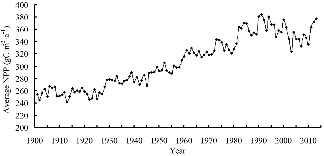
The average NPP (Fig. 1) at Heilongjiang was only 284 g C m-2 a-1 in 1901, but it reached 339 g C m-2 a-1 in 1950. Then, the average NPP decreased slightly after 1960. In the early 1980s, the average NPP of Heilongjiang began to increase rapidly. The average NPP in the early 1990s was higher than that of the other periods, reaching a peak of 414 g C m-2 a-1 in 1991. The NPP fluctuated near 375 g C m-2 a-1 in the early 21st century, and the average was 406 g C m-2 a-1 in 2013.
Fig. 1 - Average net primary production (NPP) from 1901 to 2013.
Heilongjiang was divided into three ecoregions to analyze the distribution of average NPP. The ecoregions were the Daxing’an Mountains, Xiaoxing’an Mountains, and Changbai Mountains within Heilongjiang. The highest average NPP was in the Daxing’an Mountains, and the increment was 37% from 1901 to 2013. The average NPP of the Xiaoxing’an Mountains was the lowest; however, this ecoregion had the largest increment of 45% from 1901 to 2013. The increment of average NPP in the Changbai Mountains was 39% from 1901 to 2013.
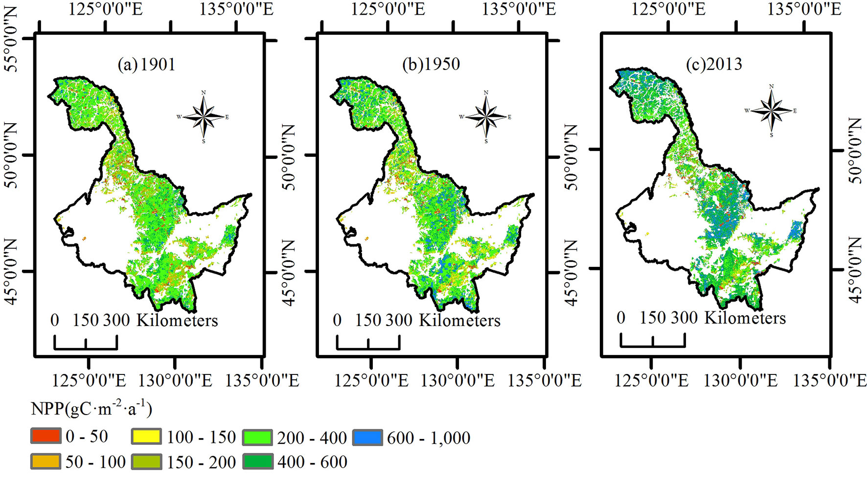
In this paper, we primarily analyzed the spatial distribution of the average NPP of the three ecoregions in 1901, 1950, and 2013 (Fig. 2). In 1901, NPP for the entire Heilongjiang region was relatively lower than that in the other years, and only the northwest region of the Daxing’an Mountains had a value higher than 400 g C m-2 a-1. In 1950, the average NPP for most of the area of the Daxing’an Mountains was between 300 and 400 g C m-2 a-1. The average NPP of the Xiaoxing’an Mountains was divided into two levels and showed an increasing trend from north to south. The average NPP of the Changbai Mountains increased in a trend from east to west. In 2013, nearly the entire Daxing’an Mountain area had an NPP value above 400 g C m-2 a-1. The NPP in the northern Xiaoxing’an Mountains increased compared with that in 1950 but was still significantly lower than that of the middle and south regions. The distribution of average NPP in the Changbai Mountains in 2013 became more uniform than that in the other years.
Fig. 2 - Spatial distribution of net primary production (NPP) in the study region of Heilongjiang. (a) 1901; (b) 1950; (c) 2013.
Results for NEP
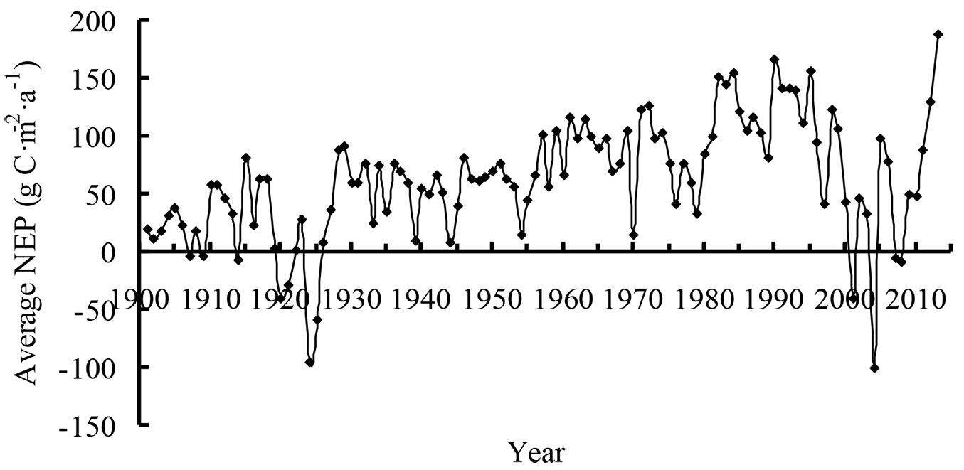
The range of average NEP in Heilongjiang was relatively large (Fig. 3). Before 1930, the average NEP fluctuated between -100 and 100 g C m-2 a-1. The minimum NEP was -95 g C m-2 a-1 in 1924. Thereafter, the average NEP began to increase gradually, and the region became a carbon sink during 1931-1949. Beginning in 1954, the NEP continued to increase until the early 1970s. However, the average NEP appeared to decrease over the long-term in the late 1970s and in the early 21st century. The average NEP increased again after 2009 and reached 188 g C m-2 a-1 in 2013.
Fig. 3 - Average net ecosystem production (NEP) from 1901 to 2013.
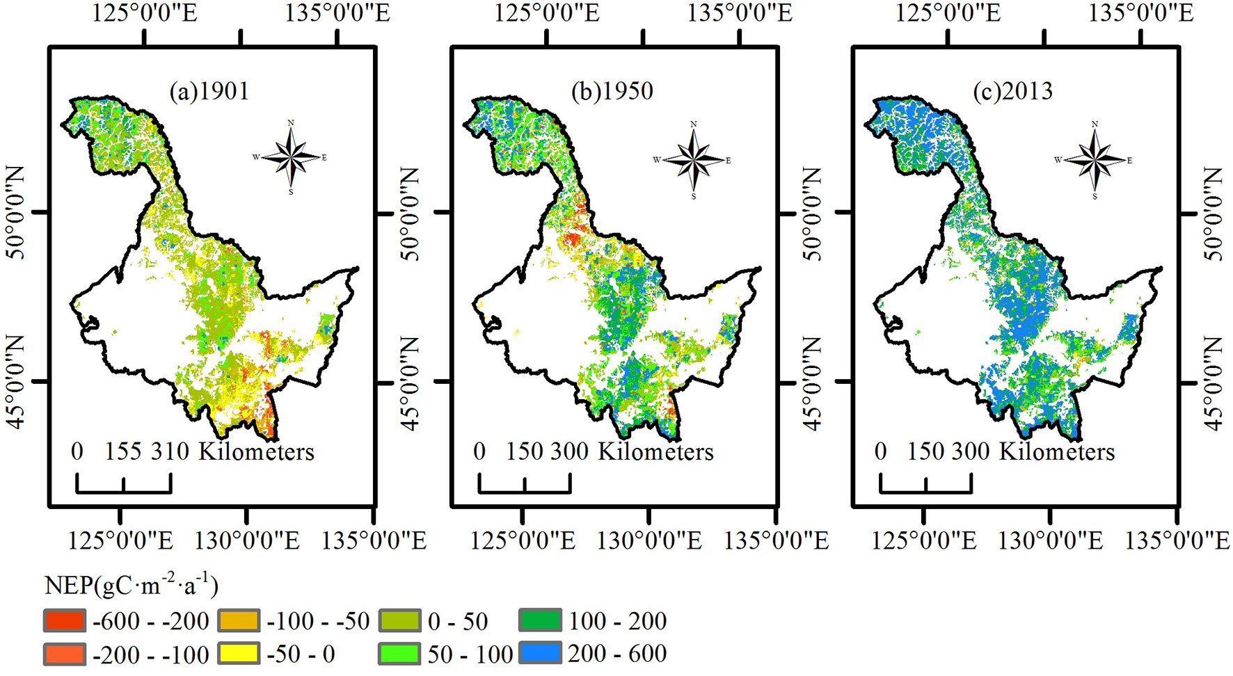
Similar to NPP, we analyzed the spatial distribution of the average NEP of three ecoregions in 1901, 1950, and 2013 (Fig. 4). In 1901, the average NEP of the Daxing’an Mountains was concentrated at a value between -100 and 100 g C m-2 a-1, with a tendency to increase from north to south. The average NEP in the Xiaoxing’an Mountains was divided into two levels; the NEP of the north region was much lower than that in the south region. Most of the Changbai Mountains had a lower NEP value than that of the other two ecoregions in 1901. In 1950, the NEP of most of the Daxing’an Mountains was between 50 and 200 g C m-2 a-1. The NEP of the south region of the Xiaoxing’an Mountains was similar to that of the Daxing’an Mountains, but the north region of the Xiaoxing’an Mountains became a carbon source, making the difference between the north and south more apparent. The entire Changbai Mountain range became more uniform than that in 1901. In 2013, the average NEP of the entire Heilongjiang region was higher than that in previous years. NEP in the north region of the Daxing’an Mountains and the south region of the Xiaoxing’an Mountains was above 200 g C m-2 a-1. The increment from 1901 to 2013 of the average NEP in the Changbai Mountains approached 200 g C m-2 a-1 and was larger than that of the other two ecoregions.
Fig. 4 - Spatial distribution of net ecosystem production (NEP) in the study region of Heilongjiang. (a) 1901; (b) 1950; (c) 2013.
Discussion
This study showed that Heilongjiang was a large C sink after 2000, which is in agreement with Wang et al. ([28]), though our result was 30% lower than that of the mentioned authors (from 1950 to 2001). The difference can be explained because only three forest types were included in their study, and the relationships between NPP and age for the different forest types were established by stand yield data for black spruce in Ontario ([5]).
Because historical eddy covariance data were not available, the simulated NEP was not comparable with annual NEE measurements at the tower flux station (45° 24.215′ N, 127° 39.651′ E - [18]). However, we validated the simulated NEP by comparison with previous studies.
In recent years, an increasing number of studies have attempted to quantify C sinks and sources for all terrestrial ecosystems in northeastern China. Zhao et al. ([39]) using the FORCCHN model reported that the total C budget in the northeast of China was between 0.11 and 0.18 Pg C a-1, and that the average C uptake was 0.15 Pg C a-1 from 1981 to 2002, which indicate that northeast China was a sink during those 22 years. Li et al. ([21]) reported that the average NEP was 22.5 g C m-2 a-1 from 1961 to 2010 based on the CEVSA model. The largest C sink occurred in the 1980s, and then the NEP declined rapidly and reached the lowest point during the late 1990s and the early 21st century. The interannual trend found in both those previous studies was consistent with that observed in our study. However, the InTEC model overestimated NEP after 1980 compared with the results of Zhao et al. ([39]) and Li et al. ([21]). These differences can be attributed to factors such as forest area, stand age information, data sources, processing methods, model structure, and effects of disturbances.
Analysis of NPP
The average NPP was low in the early 20th century and slowly increased during the following 30 years, which may have been caused by low temperatures, precipitation, atmospheric CO2 concentrations, and N deposition. Thereafter, NPP began to increase with increases in climate variability and atmospheric CO2 concentration. However, NPP began to decrease in the early 1960s because China suffered heavily from natural disasters and the Cultural Revolution in the 1960s and 1970s, when large forest areas were harvested and destroyed and large-scale plantations were uncommon ([28]). Then, the annual NPP increased rapidly and the level remained high from 1982 to 2001, which was possibly due to the Chinese government’s implementation of a series of effective policies to plant and protect forest resources ([28]). Additionally, a younger and more productive stand age structure (20-40 years old) emerged during the period.
Analysis of NEP
In this study, we analyzed the temporal variation in NEP in Heilongjiang. Heilongjiang was a carbon source in the 7 years before 1930, but was a huge carbon sink in 2013. During 1931-1949, although China suffered from the Second World War and the Chinese Civil War, Heilongjiang was not the primary battlefield, and therefore the forests in Heilongjiang were not seriously damaged. During the 113 years, two long-term reductions were apparent: one was in the late 1970s, and the other was in the early 21st century. According to the records for forest fires from 1953 to 2012 ([30]), most forest fires occurred during the same periods when long-term decreases in NEP were observed. Thus, we inferred that the disturbance factors had a large negative effect on NEP.
Uncertainty
Point-by-point comparisons between simulated NPP by BEPS and MODIS NPP in 2003 suggested that the model generally captured the magnitude of NPP in the 433 points (R2 = 0.55, RMSE = 62). Comparisons of NPP between our study and MODIS NPP also indicated that BEPS predicted NPP in the reference year reasonably well.
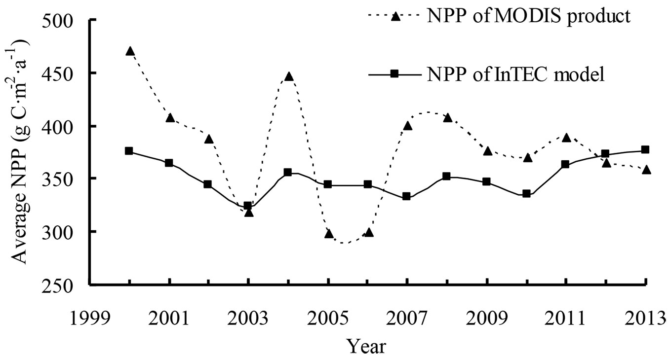
We also compared InTEC results for NPP from 2000 to 2013 with MODIS NPP (MOD17A3 - [40]). The average NPP for the period 2000-2013 in Heilongjiang forests was 379 g C m-2 a-1 and 350 g C m-2 a-1 for MODIS products and InTEC, respectively (Fig. 5). During the 14-year period, the two sources of NPP had similar patterns of change except in 2007, 2012, and 2013. Using local climate data, an average annual overestimate of 8% was found in MODIS NPP because the product was strongly driven by climate data ([22]).
Fig. 5 - Comparison of net primary production (NPP) from Integrated Terrestrial Ecosystem Carbon (InTEC) model and MODIS product from 2000 to 2013.
The National Forest Inventory data generally included age, height, diameter at breast height, stand density, species composition, and area. Based on these parameters, we calculated the biomass for different ages in sample plots using the individual biomass models produced by Ding et al. ([9], [10]). Richards’ equation was used to fit the relationship between biomass and age for each species. We estimated NPP as the sum of biomass increments or turnovers of several components as follows ([5] - eqn. 8, eqn. 9, eqn. 10):
where ΔB/Δt is the increment in the total living biomass under a particular age; M is the mortality estimated by a mean mortality rate obtained by Wang ([29]); Cb is the conversion factor of biomass to C content, which was 0.4351 for stems and roots, 0.4422 for branches, and 0.4448 for foliage ([34]); Lf is the turnover rate of foliage; Bf is the foliage biomass; Tf is the foliage (to litter) turnover ratio that differs with forest type (see Tab. 2); Cf is the ratio of carbon to dry matter, assuming Cf as 0.44 ([34]); and Lfr is the turnover rate of fine roots and the ratio of new root carbon to new leaf carbon allocation (e), which differ with forest type (Tab. 2).
Tab. 2 - Foliage turnover rates (Tf) and ratios of new fine root carbon to new leaf carbon allocation (e) for different species.
| Tree species | Tf (yr-1) | e | Reference |
|---|---|---|---|
| Pinus sylvestris var. mongolica | 0.385 | 1.03 | White et al. ([31]) |
| Larix gmelinii | 0.4 | 1.4 | White et al. ([31]) |
| Pinus koraiensis | 1 | 1.4 | White et al. ([31]) |
| Tilia amurensis | 1 | 1.2 | White et al. ([31]) |
| Betula platyphylla | 1 | 1.26 | White et al. ([31]) |
| Populus davidiana | 1 | 1.2 | White et al. ([31]) |
| Quercus mongolica | 1 | 1.2 | White et al. ([31]) |
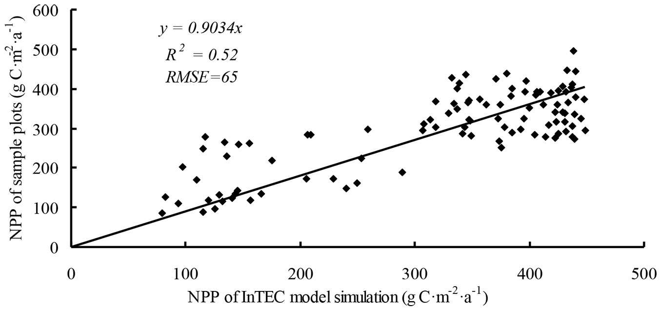
A total of 100 sample plots in the inventory data set for 2005 were used to calculate NPP and were validated by the InTEC model. InTEC slightly overestimated NPP compared with the inventory data (R2 = 0.52, RMSE = 65 - Fig. 6). The uncertainty of 25-40% was attributed to errors in the calculation of NPP and in the original data for climate, age, and NPP reference.
Fig. 6 - Comparison of calculated net primary production (NPP) from Integrated Terrestrial Ecosystem Carbon (InTEC) model and inventory plots.
We also compared simulated biomass C with previous studies from different periods in Heilongjiang. For example, Jiao & Hu ([17]) estimated the stocks of biomass C based on the forest inventory data from 1973 to 2003 (Tab. 3). Compared with those results, we observed an overestimate of biomass C by an average of 38%. The difference in forest area defined by two methods was one reason for this difference. Additionally, the forest cover type in our study was fixed and changes in forest type after disturbance were not included in our estimation.
Tab. 3 - Comparison of carbon stock in biomass from previous forest inventories with estimates in this study.
| Period | Jiao & Hu ([17]) | InTEC model | ||||
|---|---|---|---|---|---|---|
| Area (×1011 m2) |
C Pool (×1011 kg) |
C density (kg m-2) |
Area (×1011 m2) |
C Pool (×1011 kg) |
C density (kg m-2) |
|
| 1973-1976 | 2.51 | 7.96 | 3.17 | 1.88 | 6.92 | 3.70 |
| 1977-1981 | 1.53 | 5.41 | 3.55 | 1.88 | 7.29 | 3.90 |
| 1984-1988 | 1.56 | 5.66 | 3.64 | 1.88 | 8.23 | 4.40 |
| 1989-1993 | 1.61 | 5.88 | 3.65 | 1.88 | 8.60 | 4.60 |
| 1994-1998 | 1.76 | 6.22 | 3.54 | 1.88 | 9.35 | 5.00 |
| 1999-2003 | 1.80 | 6.01 | 3.34 | 1.88 | 9.72 | 5.20 |
Similarly, we compared the soil C stock with that in other studies. However, because the definitions of forest area, cover type, and soil depth were different between the InTEC model and those in other studies, comparisons of the results for soil C storage were difficult. Comparisons of the estimates of soil C density between our study and those in others indicated that the InTEC model simulated C changes in soil reasonably well (Tab. 4), although the model slightly underestimated soil C density.
Tab. 4 - Comparison of carbon stock in soil from previous forest inventories with the estimates obtained in this study.
| Value in this study (kg m-2) |
Estimate (kg m-2) |
Method | Period | Region | Reference |
|---|---|---|---|---|---|
| 13.27 | 13.57 | Based on the Second National Soil Survey | 1980s | Heilongjiang | Fang et al. ([12]) |
| 13.30 | 21.78 | FORCCHN model | 1981-2002 | Northeast China | Zhao et al. ([39]) |
| 13.33 | 14.70 | Based on multi-purpose regional geochemical survey | 2006 | Heilongjiang | Xi et al. ([32]) |
| 17.38 | 17.26 | Based on the date plots measured | 2008-2011 | Daxing’an Mountains of Heilongjiang | Hong ([16]) |
| 12.67 | 16.79 | Based on the date plots measured | 2008-2011 | Xiaoxing’an Mountains of Heilongjiang | Hong ([16]) |
Conclusions
In this paper, we used the InTEC model to estimate NPP and NEP in Heilongjiang from 1901 to 2013 and then analyzed the dynamic changes in the spatiotemporal C balance over the 113 years.
Our analysis indicated that NPP was low in the early 20th century; thereafter, NPP began to increase steadily and reached peak values in the early 1990s. Recently, NPP has been maintained at a relatively high level between 390 g C m-2 a-1 and 410 g C m-2 a-1. We concluded that NPP was closely related to climate change and the length of the growing season. However, greater efforts toward forest protection and a more reasonable stand age structure were the decisive factors for the increase in NPP in Heilongjiang.
The average NEP of Heilongjiang varied greatly, but we found that most forest disturbances occurred in the identical periods as long-term decreases in NEP. Disturbances periodically released large amounts of C to the atmosphere and further changed stand age structures. Our study showed that NEP in Heilongjiang forests was greatly influenced by disturbance factors, which is consistent with previous studies ([36]). Reducing the occurrence of disturbances, particularly fire, will maintain a high level of NEP in Heilongjiang.
According to the spatial distribution of NPP in Heilongjiang in 1901, 1950, and 2013, NPP in the Xiaoxing’an Mountains showed a tendency to increase from north to south, which is consistent with the distribution of forest coverage. The distribution of NPP in the Changbai Mountains was more uniform than that of the Xiaoxing’an Mountains; however, the lowest average NPP was in these mountains. The spatial distribution of NEP was similar to that of NPP in Heilongjiang. We believe that this result was due to low forest coverage; therefore, large-scale forest plantations in these two regions will improve both NPP and NEP.
In this study, a method was used that estimated the distribution of the C balance in Heilongjiang and quantitatively analyzed the changes in spatiotemporal C budgets by offering a reference to assess the C balance in the past and project the variation into the future. Some aspects of this study were inadequate; for example, effects of disturbances were determined by changes in forest stand age structure rather than separating the disturbances into harvests, insect attacks, and fires. Furthermore, the 1 km resolution was too coarse to adequately explore the C dynamics in each pixel, because numerous pixels were mixed with nonforest plants. Additionally, the lack of available historical eddy covariance data resulted in insufficient validation of NEP. Hence, these aspects of the estimates of the C budgets of Heilongjiang will be addressed in future studies.
Acknowledgments
Research grants from the National Natural Science Foundation of China (31470640 and 31300420), the Natural Science Foundation of Jiangsu (BK20130987) and the Fundamental Research Funds for the Central Universities (2572016AA30) supported this research. Models in support of this article were from the research collaboration with Prof. Jingming Chen and Fangmin Zhang at the University of Toronto; please contact the authors for more details.
References
Gscholar
Gscholar
Gscholar
Gscholar
CrossRef | Gscholar
Gscholar
Gscholar
Gscholar
Gscholar
Gscholar
Gscholar
Gscholar
CrossRef | Gscholar
Authors’ Info
Authors’ Affiliation
Collaborative Innovation Center on Forecast and Evaluation of Meteorological Disasters, College of Applied Meteorology, Nanjing University of Information Science and Technology, Nanjing, Jiangsu, 210044 (P.R. China)
Corresponding author
Paper Info
Citation
Wang B, Li M, Fan W, Zhang F (2016). Quantitative simulation of C budgets in a forest in Heilongjiang province, China. iForest 10: 128-135. - doi: 10.3832/ifor1918-009
Academic Editor
Chris Eastaugh
Paper history
Received: Nov 15, 2015
Accepted: Aug 22, 2016
First online: Nov 06, 2016
Publication Date: Feb 28, 2017
Publication Time: 2.53 months
Copyright Information
© SISEF - The Italian Society of Silviculture and Forest Ecology 2016
Open Access
This article is distributed under the terms of the Creative Commons Attribution-Non Commercial 4.0 International (https://creativecommons.org/licenses/by-nc/4.0/), which permits unrestricted use, distribution, and reproduction in any medium, provided you give appropriate credit to the original author(s) and the source, provide a link to the Creative Commons license, and indicate if changes were made.

Web Metrics
Breakdown by View Type
Article Usage
Total Article Views: 48816
(from publication date up to now)
Breakdown by View Type
HTML Page Views: 40691
Abstract Page Views: 2965
PDF Downloads: 3729
Citation/Reference Downloads: 58
XML Downloads: 1373
Web Metrics
Days since publication: 3544
Overall contacts: 48816
Avg. contacts per week: 96.42
Article Citations
Article citations are based on data periodically collected from the Clarivate Web of Science web site
(last update: Mar 2025)
Total number of cites (since 2017): 6
Average cites per year: 0.67
Publication Metrics
by Dimensions ©
Articles citing this article
List of the papers citing this article based on CrossRef Cited-by.
Related Contents
iForest Similar Articles
Short Communications
Hydrology, element budgets, acidification, nutrient N in a climate change perspective for the northern forest region
vol. 2, pp. 23-25 (online: 21 January 2009)
Research Articles
Potential impacts of regional climate change on site productivity of Larix olgensis plantations in northeast China
vol. 8, pp. 642-651 (online: 02 March 2015)
Research Articles
Model-based assessment of ecological adaptations of three forest tree species growing in Italy and impact on carbon and water balance at national scale under current and future climate scenarios
vol. 5, pp. 235-246 (online: 24 October 2012)
Research Articles
Predicting the effect of climate change on tree species abundance and distribution at a regional scale
vol. 1, pp. 132-139 (online: 27 August 2008)
Research Articles
Seeing, believing, acting: climate change attitudes and adaptation of Hungarian forest managers
vol. 15, pp. 509-518 (online: 14 December 2022)
Research Articles
An assessment of climate change impacts on the tropical forests of Central America using the Holdridge Life Zone (HLZ) land classification system
vol. 6, pp. 183-189 (online: 08 May 2013)
Research Articles
Impacts of stump harvesting on carbon dioxide, methane and nitrous oxide fluxes
vol. 15, pp. 148-162 (online: 07 May 2022)
Research Articles
Is Pinus pinea growth affected by climate change in western Anatolia?
vol. 18, pp. 93-101 (online: 28 April 2025)
Research Articles
Impact of climate change on radial growth of Siberian spruce and Scots pine in North-western Russia
vol. 1, pp. 13-21 (online: 28 February 2008)
Review Papers
Impacts of climate change on the establishment, distribution, growth and mortality of Swiss stone pine (Pinus cembra L.)
vol. 3, pp. 82-85 (online: 15 July 2010)
iForest Database Search
Search By Author
Search By Keyword
Google Scholar Search
Citing Articles
Search By Author
Search By Keywords
PubMed Search
Search By Author
Search By Keyword


