Determining Pleiades satellite data capability for tree diversity modeling
iForest - Biogeosciences and Forestry, Volume 10, Issue 1, Pages 348-352 (2016)
doi: https://doi.org/10.3832/ifor1884-009
Published: Nov 19, 2016 - Copyright © 2016 SISEF
Short Communications
Abstract
Modeling of the spatial distribution of tree species based on survey data has recently been applied to conservation planning. Numerous methods have been developed for building species habitat suitability models. The aim of this study was to investigate the suitability of Pleiades satellite data for modeling tree species diversity of Hyrcanian forests in northern Iran (Mazandaran Province). One-hundred sample plots were established over an area of 2.600 ha and surveyed for tree diversity, and the Simpson’s index (D), Shannon’s index (H’) and the reciprocal of Simpson’s index (1/D) were calculated for each plot. Spectral variables and several parameters derived by texture analysis were obtained from multispectral images of the study area and used as predictors of tree diversity of sample plots. Two different methods, including generalized additive models (GAMs) and multivariate adaptive regression splines (MARS), were used for modeling. The results revealed a fairly good prediction of plot tree diversity obtained using the developed models (adj-R2 = 0.542-0.731). Shannon’s H’ and Simpson’s 1/D indices were more accurately predicted using GAM-based methods, while MARS models were more suitable for predicting Simpson’s D. We concluded that Pleiades satellite data can be conveniently used for estimating, assessing and monitoring tree species diversity in the mixed hardwood Hyrcanian forest of northern Iran.
Keywords
Pleiades, Tree Species Diversity, Modeling, Darabkola Forest
Introduction
The exponential increase of the world population in the last decades has brought about an unparalleled human exploitation of natural resources worldwide, leading to a global reduction of the naturalness of many environments. This may result in the reduction of biodiversity as well as environmental functions and ecological processes which act to generate and maintain soils, convert solar energy into plant tissue, regulate climatic parameters, and provide multiple forest products ([14]). The Hyrcanian forest is the natural ecosystem with the highest plant and animal diversity in Iran. However, these forests are being more and more impoverished by degradation and conversion to other land uses. Moreover, increasing and maintaining the structural diversity in forest stands has become an important forest management strategy to face the climate change.
Accurate and practical methods for estimating biodiversity are needed to develop effective strategies for the conservation and management of forests ([12]). In recent years, the increased spatial and spectral resolution of remote sensors has made it increasingly feasible to conduct direct mapping of biodiversity through mapping plant and tree canopies and assemblages, and in some cases, through the identification of individual species of trees. Recent studies have indicated that remote sensing has a high capability of providing useful information on biodiversity ([12], [17], [24], [22]). Numerous remotely-detected parameters can be used as proxies of the occurrence, distribution and abundance of species. Remotely sensed data allow to quantify net primary productivity (NPP) through the Normalized Difference Vegetation Index (NDVI). This index has shown to be either positively or negatively associated with NPP, depending on the scale ([31]). Also, NDVI has been used in several studies for modeling species occurrence ([18]) or species richness at regional and local scales ([25], [7]). A further factor related to species richness is the structural and compositional complexity of habitats, which can be measured by either the variability of spectral indices (such as NDVI) or a band in the immediate neighborhood of each sampling unit, or using approaches that calculate spectral variability using multiple bands ([28], [26]). Such a spectral variability is directly related to the heterogeneity of resource distribution (mixed habitats), which may be assessed by analyzing the variability in the reflectance values among pixels using the texture of a remotely sensed image ([10]). Mohammadi & Shataee ([22]) investigated the possibility to estimate tree diversity using Landsat Enhanced Thematic Mapper Plus (ETM+) satellite data in the Hyrcanian forests of the Golestan Province in Iran. Kalbi et al. ([16]) compared two nonparametric methods such as the classification and regression tree (CART) and Random forest (RF) for predicting tree diversity distribution using the High Resolution Geometric sensor (HRG) of earth-observing satellites (SPOT-HRG) data. Bawa et al. ([4]) reported a statistically significant relationship between species diversity and the normalized difference vegetation index (NDVI) derived from Indian Remote Sensing Satellite (IRS-1C) imagery, so that NDVI may be used to characterize areas of high and low tree species richness in tropical forests where biodiversity loss is high. Moreover, regression analysis approaches have been broadly applied in ecological surveys ([19], [5], [32]). Regression approaches have proven particularly useful in modeling the spatial distribution of species and communities ([9]). The development of advanced nonparametric regression and machine learning techniques are opening up many opportunities for modeling tree diversity of greater accuracy compared with linear regression ([2]). Recently, generalized linear models ([19]) and generalized additive models ([11]) using presence-absence survey data have also been given much more attention. Presence-absence niche models use algorithms that can model the presence or the absence of a species as binary response. Moisen & Frescino ([23]) investigated the performance of non-parametric techniques such as CART, generalized additive models (GAM) and artificial neural networks (ANN) and compared them to parametric techniques for the prediction of several species-independent forest characteristics in the interior western United States. MARS and ANN models seemed to work best when applied to simulated data, though their application to real data appeared less suitable, in which case a linear modeling (LM) approach often provided comparable results. Overall, GAMs and MARS were marginally best for modeling forest characteristics.
The aim of this study was to: (i) investgate the relationships between field-based tree diversity and the spectral and textural features of remote-sensed data (multispectral images of Pleiades satellite); (ii) compare two statistical non-parametric techniques (GAM and MARS) for modeling tree species diversity.
Materials and methods
Study area
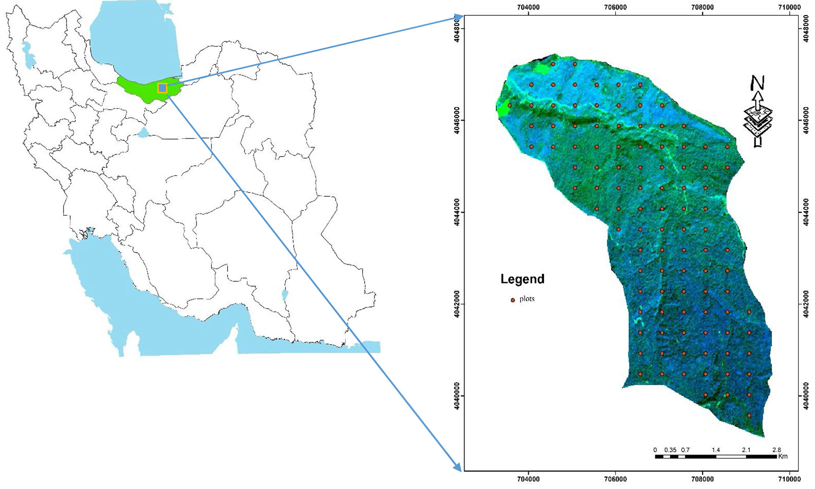
The study area is located within the Hyrcanian forests, District 1 of Darabkola’s forests, Sari, northern Iran (lat. 36° 28’ - 36° 33′ N, long. 53° 16′ - 53° 20′ W - Fig. 1). The Darabkola forest covers about 2.600 hectares and consists of natural temperate and uneven aged stands. The main tree species are Quercus castaneafolia (chestnut-leaved oak), Carpinus betulus (hornbeam), Acer velutinum (velvet maple), Alnus subcordata (Caucasian alder), Tilia begonifolia (linden tree), Parrotia persica (Persian parotia), Ulmus glabra (wych elm), Acer platanoides (Norway maple), Diospyros lotus (date pulm), Zelkova carpinifolia (Siberian elm), Fagus orientalis (Oriental beech) and Acer cappadocicum (coliseum maple).
Fig. 1 - Location of the study area in the Mazandaran Province, northern Iran (left panel) and distribution of the sample plots in the study area (right panel).
Field data
As species richness and diversity indices depend on the size of the sample plot, phytosociological data were collected based on a systematic sampling method during the period 5 June to 15 July 2010. The size and the number of quadrats were determined based on the species area curve ([21]). The choice of the sample size and the number of sampling units to select is a key part of planning a survey. One hundred square-shaped sample plots (60 × 60 m) were placed over the study area using a stratified systematic sampling and an overlying grid of 450 × 500 m (see Fig. 1, right panel). For each plot, the main characteristics (species, tree health, etc.) of trees with a diameter at breast height (DBH) greater than 7.5 cm were measured. The geographic coordinates of each plot center were recorded using a Trimble 3 DGPS receiver.
The Simpson’s diversity index (D), the Shannon’s diversity index (H′), and the reciprocal of Simpson’s diversity index (1/D) were calculated for each sampling plot based on the proportion of tree species recorded during the field survey. Other indices commonly used for describing the forest structural diversity or the dissimilarity of species across the landscape (e.g., mingling index, coefficient of segregation, etc. - [27], [3], [13]) were not considered in this study.
Preprocessing and processing of satellite images
Multispectral images of the Pleiades satellite (Airbus Defence and Space, Munich, Germany - ⇒ http://www.intelligence-airbusds.com/pleiades/) were acquired in April 2013. All images had a 16-bit radiometric resolution. Geometric correction and orthorectification were applied to images before their use. The geometrical correction of the images was optimized by comparing the image data with vector layers of the roads in the studied area.
Pleiades satellite images have four spectral bands (Blue, Red, Green and NIR) with a spatial resolution of 2 m and a panchromatic (PAN) band with a resolution of 0.5 m. In this study, we considered the aforementioned four spectral bands, the PAN band, the Normalized Difference Vegetation Index (NDVI), and the derived texture features of these bands as predictors in the model analysis (Tab. 1).
Tab. 1 - Overview of the predictor variables selected by the tree biodiversity models developed in this study.
| Tree Diversity Index |
Modeling technique |
Variables selected by the model |
|---|---|---|
| Simpson’s D | GAM | Mean NIR, Mean Red, Variance NDVI, Contrast NIR |
| MARS | Entropy NIR, NDVI, NIR, Mean NIR | |
| Shannon’s H′ | GAM | Mean Green, Mean Red, Variance NIR, Contrast NIR |
| MARS | Mean NIR, NIR, Dissimilarity Red | |
| Simpson’s 1/D | GAM | Mean Red, Variance Green, Variance NIR, Mean Red, |
| MARS | Mean NIR, Contrast Red, Entropy NIR |
Texture analysis is one of the most suitable processing methods to estimate the characteristics of the forest structure from remote-sensed data ([15]). It can be applied to estimate local softness, roughness, smoothness and regularity of each variable based on the spatial variation of its pixel values ([9]). For each variable considered in this study, several parameters were derived by texture analysis, such as mean, variance, entropy, dissimilarity, homogeneity, angular second moment, correlation and grey-level-difference vector ([6], [29], [30]). Texture analysis was carried out over the study area using multiple window sizes (9×9, 11×11, 13×13, 15×15 and 17×17 pixels), in order to define the area used for statistical calculations.
All the above derived parameters were calculated over the whole study area at the original pixel resolution.
Spectral signature extraction of the plots
All the images (for both the original variables and the derived parameters) were aggregated at a resolution of 60 m (consistently with the size of the field plots - 60×60 m) and their pixel values averaged. Average values for each variable were then extracted from the location of each field plot.
Statistical models
Generalized additive models
Generalized additive models (GAMs) are semi-parametric regression models ([11]). Response curves in GAMs are estimated with smoothing functions, allowing a wide range of response curves to be fitted to the input data ([33]). The main advantage of GAM is its ability to deal with highly non-linear and non-monotonic relationships between the response variable and a set of explanatory variables. Thus, GAMs are sometimes referred to as a data-driven rather than model-driven process ([9]). Being N the number of observations and p the number of explanatory variables, the generalized additive model is defined as (eqn. 1):
where fj are smoothed functions estimated from input data, μ represents the expected value, G is the link function, and i = 1, 2, 3, …, N. These functions are based on the assumption that E[fj(xj)] = 0 (j = 1, 2, …, N). In such a model, the dependent variable can be non-Gaussian and not necessarily continuous in nature, thereby allowing the construction of more flexible models.
Multivariate adaptive regression splines (MARS)
The multivariate adaptive regression spline (MARS) method was first introduced by Friedman & Stueltze ([8]) to overcome some limitations of the regression trees. MARS is a regression method that is suitable to high dimensional data. The MARS procedure builds flexible regression models by using basis functions to fit separate splines to distinct intervals (ranges) of the input predictor variables. Both the variables in use and the end points of the intervals (knots), are located using an exhaustive search procedure that relies on a special class of basic functions ([1]). MARS models the target variable using a linear combination of splines, which are automatically built (matching the boundaries of each region) from an increasing set of piecewise-defined linear basic functions ([23]). MARS automatically selects the amount of smoothing required for each predictor as well as the interaction order of the predictors. It is considered a projection method where variable selection is not of concern, though the maximum level of interaction has to be determined. We considered 15 variants of these models formed by different combinations of the parameter nk that sets the maximum number of terms before pruning; two variants (1 and 2) of the parameter degree that sets the maximum degree of interaction; and four variants (0.01, 0.001, 0.005 and 0.0005) of the parameter thresh specifying the forward stepwise stopping threshold.
Model evaluation and performance assessment
The available data were randomly split into two subsets, 70% of the data for modeling and 30% for validation and testing. For each tested model, several statistics were recorded, including the squared coefficient of determination (R2) and the adjusted coefficient of determination (adjusted R2). The latter was used to estimate the expected shrinkage in R2 due to over-fitting and the inclusion of too many independent variables in the regression model. Thus, when the adjusted R2 value is much lower than the R2 value, the regression may be over-fitted to the sample, and therefore poorly generalizable.
Model performances were assessed on the validation subset using several regression diagnostics metrics such as the root mean square error (RMSE), relative RMSE, bias and relative bias, calculated as follows (eqn. 2 to eqn. 5):
where esti is the value predicted by the model at the i-th pixel of the validation subset, obsi is the observed values at the same pixel and m is the number of pixels in the validation subset. In addition, some common graphical diagnostic tools ([20]) were used to evaluate the quality of model performances.
Results
A high tree species diversity was observed in the study area, as inferred from the three diversity indices obtained from the field survey. The main descriptive statistics of the Simpson’s diversity index (D), the Shannon’s diversity index (H’), and the reciprocal of the Simpson’s diversity index (1/D) in the two datasets (training and validation subsets) are reported in Tab. 2. Overall, D varied between 0.105 to 0.86 across the analyzed sample plots, while H’ ranged from 0.12 to 2.56 and 1/D ranged from 1.105 to 4.02.
Tab. 2 - Descriptive statistics of model and validation samples for indices. (SD): standard deviation.
| Tree Diversity Index |
Training Dataset | Validation Dataset | ||||||||
|---|---|---|---|---|---|---|---|---|---|---|
| N | Mean | Min | Max | SD | N | Mean | Min | Max | SD | |
| Simpson’s D | 70 | 0.47 | 0.11 | 0.76 | 0.17 | 30 | 0.57 | 0.13 | 0.76 | 0.12 |
| Shannon’s H′ | 70 | 1.28 | 0.12 | 2.56 | 0.47 | 30 | 1.49 | 0.14 | 2.17 | 0.41 |
| Simpson’s 1/D | 70 | 2.11 | 1.10 | 4.01 | 0.64 | 30 | 2.50 | 1.24 | 3.94 | 0.63 |
Regarding the window size used for texture analysis, the highest correlation between texture-derived parameters and all tree diversity indexes was found using the window size 9×9 pixels, which was then used in modeling to extrapolate the texture features of the analyzed spectral variables.
All the models were critically investigated for confounding factors and checked for all basic assumptions. The number of predictor variables entering the models ranged from two to eight, differing among both the models and the diversity indices considered. For example, regarding the index D, the best predictors were: NIR (mean and contrast), Red, and NDVI (variance) using the GAM models; and NIR (mean and entropy) and NDVI using the MARS model (Tab. 1). Overall, NIR (both as variable and its texture-analysis derived parameters) was the most represented predictor across models and indices (12 times), followed by Red (6 times), and NDVI and Green band (both 2 times).
The performance statistics for each model are summarized in Tab. 3. The proportion of the total variance accounted for by the different models (as inferred from the adj-R2 values) ranged from 54.2% (MARS, 1/D) to 73.1% (MARS, D), indicating a fairly good predicting ability of the models.
Tab. 3 - Performance indices of all SI-models for the three tree species and five modelling techniques. (*): best model performance for every evaluation measure.
| Tree Diversity Index |
Modeling technique |
R2 | R2adj | RMSE | RMSE% | Bias | Bias% |
|---|---|---|---|---|---|---|---|
| Simpson’s D | GAM | 0.623 | 0.617 | 0.92 | 20.7 | 0.01 | 2.6 |
| MARS* | 0.743 | 0.731 | 0.08 | 18.6 | -0.01 | -2.6 | |
| Shannon’s H′ | GAM* | 0.624 | 0.621 | 0.37 | 29.8 | -0.17 | -13.7 |
| MARS | 0.563 | 0.542 | 0.5 | 40.32 | -0.22 | -18.2 | |
| Simpson’s 1/D | GAM* | 0.653 | 0.646 | 0.30 | 24.19 | -0.14 | -11.2 |
| MARS | 0.615 | 0.59 | 0.52 | 41.9 | -0.23 | -18.5 |
The best model performance was evaluated based on the highest R2, highest adjusted R2 and lowest RMSE, RMSEr Bias and Biasr values. In the most cases, the best goodness-of-fit between the predicted and the observed tree diversity index values at the field plots was obtained by the GAM, which had the lowest values for RMSE and Bias and the highest adjusted R2. However, the best fitting was obtained when the tree diversity MARS model was used to predict the Simpson’s index D.
Discussion
Hyrcanian forests of northern Iran comprise a highly diverse vegetation cover and are increasingly degraded and converted to other land uses. Understanding the main factors that influence the spatial distribution of both local species richness and spatial species turnover is important to adequately map tree diversity. In this study, we assessed the utility of Pleiades satellite image data and two regression techniques for modeling tree diversity in a Hyrcanian Forest. These results are similar to those obtained by other studies aimed at identifying broad patterns of tree species diversity by satellite data ([12], [22], [32]).
All the statistical models applied in this study provided fairly successful predictions of forest tree diversity based on remote-sensed data. In particular, GAM and MARS modeling regressions were successfully applied to identify those parts of the study area where tree species richness is above the average. In a comparable study, Wang et al. ([32]) report that GAM performed better and showed a better adaptability to extreme observations than other non-linear and non-parametric techniques, according to previous studies ([2]). Brenning ([5]) showed that the application of simple models, such as GAM, are similarly successful as compared with complex machine learning techniques. Our study confirm these findings, as GAM models provided in most cases a better fitting than MARS based on most evaluation measures.
The results of this study are not directly comparable with other relevant researches in particular regarding the use of variables derived by texture analysis as predictors. Furthermore, most studies published in the literature used satellite imagery with different spectral/spatial resolutions and/or were conducted in different forest conditions.
Our results showed that Pleiades satellite data and non-parametric regression models could be conveniently used by resource manager to achieve useful indications on tree diversity distribution over large areas in northeastern Iran, as well as to assess and monitor the status of tree diversity of Hyrcanian forests.
A strong limitation faced by conservation biologists and managers of natural resources is the lack of information concerning species distribution patterns. To this purpose, precise biodiversity mapping produced by accurate modeling could help in the selection and effectiveness of protected natural areas.
References
Gscholar
Gscholar
Gscholar
Gscholar
Authors’ Info
Authors’ Affiliation
Siavash Kalbi
Sari Agriculture and Natural Resource University, Forestry Department, Sari 578 (Iran)
Corresponding author
Paper Info
Citation
Akbari H, Kalbi S (2016). Determining Pleiades satellite data capability for tree diversity modeling. iForest 10: 348-352. - doi: 10.3832/ifor1884-009
Academic Editor
Alessandro Montaghi
Paper history
Received: Sep 27, 2015
Accepted: Jul 18, 2016
First online: Nov 19, 2016
Publication Date: Feb 28, 2017
Publication Time: 4.13 months
Copyright Information
© SISEF - The Italian Society of Silviculture and Forest Ecology 2016
Open Access
This article is distributed under the terms of the Creative Commons Attribution-Non Commercial 4.0 International (https://creativecommons.org/licenses/by-nc/4.0/), which permits unrestricted use, distribution, and reproduction in any medium, provided you give appropriate credit to the original author(s) and the source, provide a link to the Creative Commons license, and indicate if changes were made.

Web Metrics
Breakdown by View Type
Article Usage
Total Article Views: 49453
(from publication date up to now)
Breakdown by View Type
HTML Page Views: 41097
Abstract Page Views: 3059
PDF Downloads: 3953
Citation/Reference Downloads: 50
XML Downloads: 1294
Web Metrics
Days since publication: 3491
Overall contacts: 49453
Avg. contacts per week: 99.16
Article Citations
Article citations are based on data periodically collected from the Clarivate Web of Science web site
(last update: Mar 2025)
Total number of cites (since 2017): 3
Average cites per year: 0.33
Publication Metrics
by Dimensions ©
Articles citing this article
List of the papers citing this article based on CrossRef Cited-by.
Related Contents
iForest Similar Articles
Review Papers
Remote sensing-supported vegetation parameters for regional climate models: a brief review
vol. 3, pp. 98-101 (online: 15 July 2010)
Review Papers
Accuracy of determining specific parameters of the urban forest using remote sensing
vol. 12, pp. 498-510 (online: 02 December 2019)
Technical Reports
Detecting tree water deficit by very low altitude remote sensing
vol. 10, pp. 215-219 (online: 11 February 2017)
Review Papers
Remote sensing of selective logging in tropical forests: current state and future directions
vol. 13, pp. 286-300 (online: 10 July 2020)
Research Articles
Assessing water quality by remote sensing in small lakes: the case study of Monticchio lakes in southern Italy
vol. 2, pp. 154-161 (online: 30 July 2009)
Research Articles
Afforestation monitoring through automatic analysis of 36-years Landsat Best Available Composites
vol. 15, pp. 220-228 (online: 12 July 2022)
Technical Reports
Remote sensing of american maple in alluvial forests: a case study in an island complex of the Loire valley (France)
vol. 13, pp. 409-416 (online: 16 September 2020)
Review Papers
Remote sensing support for post fire forest management
vol. 1, pp. 6-12 (online: 28 February 2008)
Research Articles
Development of monitoring methods for Hemlock Woolly Adelgid induced tree mortality within a Southern Appalachian landscape with inhibited access
vol. 9, pp. 178-186 (online: 02 January 2016)
Research Articles
Classification of xeric scrub forest species using machine learning and optical and LiDAR drone data capture
vol. 18, pp. 357-365 (online: 07 December 2025)
iForest Database Search
Search By Author
Search By Keyword
Google Scholar Search
Citing Articles
Search By Author
Search By Keywords
PubMed Search
Search By Author
Search By Keyword


