
Carbon and water vapor balance in a subtropical pine plantation
iForest - Biogeosciences and Forestry, Volume 9, Issue 5, Pages 736-742 (2016)
doi: https://doi.org/10.3832/ifor1815-009
Published: May 25, 2016 - Copyright © 2016 SISEF
Research Articles
Abstract
Afforestation has been proposed as an effective tool for protecting primary and/or secondary forests and for mitigating atmospheric CO2. However, the dynamics of primary productivity differs between plantations and natural forests. The objective of this work was to evaluate the potential for carbon storage of a commercial pine plantation by determining its carbon balance. Measurements started when trees were aged 6 and ended when they were older than 8 years. We measured CO2 and water vapor concentrations using the Eddy covariance method. Gross primary productivity in 2010 and 2011 was 4290 ± 473 g C m-2 and 4015 ± 485 g C m-2, respectively. Ecosystem respiration ranged between 7 and 20 g C m-2 d-1, reaching peaks in all Februaries. Of the 30 months monitored, the plantation acted as carbon source for 21 months and as carbon sink for 6 months, while values close to neutrality were obtained during 3 months. The positive balance representing CO2 loss by the system was most likely due to the cut branches left on the ground following pruning activities. The plantation was subjected to pruning in January and September 2008 and to sanitary pruning in October 2010. In all cases, cut branches were not removed but remained on the ground. Residue management seems to have a very important impact on carbon balance.
Keywords
Afforestation, Carbon Source, Ecosystem Respiration, Pruning, Thinning
Introduction
Land use change is highly responsible for the increase in the concentration of greenhouse gases (GHGs) in the atmosphere, thus having an important impact on the regional climate ([41], [16]). The growth of the world’s population has increased the demand for agricultural land, leading to more pressure on forests. These are estimated to store about 45% of the terrestrial carbon, contributing to 50% of the net primary production ([37]). Therefore, the reduction of forests is expected to dramatically impact the balance of atmospheric CO2. Mid-latitude forests are among the most modified ecosystems over the last century, but current land-use change models predict increased over-exploitation of tropical forests ([43]). The conservation of forest resources appears as a reasonable option for mitigating the concentration of greenhouse gases (GHGs) in the atmosphere ([29], [25]). Afforestation has been proposed as an effective tool for protecting primary and/or secondary forests and for mitigating atmospheric CO2 levels ([40], [35], [18]).
The dynamics of primary productivity in plantations differs from that of native forests, as it depends on the age of the stands, the species planted, soil type, climate and management practices ([33]), while that of native forests depends directly on the age of the trees ([30]). Plantation stands are capable of producing high biomass yields, but they are exposed to continuous disturbances (e.g., field preparation, fertilization, weed control, thinning and harvest) which may possibly affect CO2 uptake. Only a few studies conducted in forest systems have included large woody debris such as branches in the analysis of carbon flux because of their low decomposition rate ([6]). Overall, commercial plantations have been less studied than natural forests. Noormets et al. ([31]) reported high values of gross productivity, and high values of soil and litter respiration in a 25 years-old pine plantation. Paul et al. ([34]) found that carbon losses occur within the first 10 years after the establishment of the plantation, while 30 years are required to restore the initial levels. The impact of afforestation on the global carbon budget has become increasingly important due to the expansion of plantation areas. McKinley et al. ([25]) estimated that plantations are responsible for 50% of carbon uptake by forests of USA.
The estimation of carbon balance in plantations is a challenge because of the slowness of soil cycling processes, the spatial heterogeneity of soils and the low rate of tree growth. The eddy covariance technique allows direct estimation of the exchange of matter and energy between an ecosystem and the atmosphere ([1], [3]). It is used to measure net ecosystem CO2 exchange (NEE), even for short periods of time, providing information on entire ecosystems over surface areas of the order of hundreds of square meters ([38]). Moreover, this is a highly robust method because fluxes are obtained almost continuously on timescales ranging from half hours to multiple years. Globally, over 500 eddy covariance flux towers are currently operating (⇒ http://www.fluxnet.ornl.gov/). Most of these are located in the United States and Europe, while countries of the Southern Hemisphere are poorly represented. Furthermore, the forests sites included in the Fluxnet network often correspond to native forests undisturbed or undergoing restoration.
The present study reports eddy covariance measurements carried out during the first rotation of a commercial pine plantation. Measurements started when trees were 6 years old and lasted for 2.5 years. The plantation was subjected to pruning in January and September 2008, and to sanitary pruning in October 2010. In all these occasions, cut branches were not removed from the ground. Our main objective was to determine the net ecosystem CO2 and water vapor exchange to assess the potential of the pine plantation for carbon storage, in the context of residue practices.
Material and methods
Study area
The study was conducted in a commercial Pinus taeda plantation, near the locality of Virasoro, Corrientes province, Argentina (28° 14′ 22.2″ S, 56° 11′ 19.11″ W), between December 2009 and May 2012. The stands were located on a gentle hillock at elevation 127 m a.s.l. The region has a subtropical climate without a dry season. Mean annual rainfall is 1800 mm, and mean temperature is 21.1 °C, with mean maximum and minimum temperatures of 26.5 °C and 15.7 °C, respectively (historical data for the period 1980-2010, National Weather Service). Mean air humidity is 72%. The soils belong to the Ultisols order (Kandihumult), with clayish texture, good drainage, and a depth of about 150 cm (INTA Soil Map at a 1:500.000 scale). The plantation forest was set up in 2003, replacing natural grasslands. It was subjected to pruning in January and September 2008 and to sanitary pruning in October 2010 due to infestation by wood wasp Sirex noctilio, a pest of pine trees. On these occasions, cut branches were left on the forest floor. Measurements started when trees were 6 years old and 12 m in height. The tower equipped with instruments was surrounded by at least 700 m of homogeneous forest in all directions.
Instruments
Instruments were installed on a 32-m fire surveillance tower at 18 m above the ground and at 6 m above the canopy. The tower is property of Forestal Bosques del Plata S.A. (⇒ http://www.bosquesdelplata.com.ar). We used a 3-D sonic anemometer (CSAT3®, Campbell Scientific, Logan, Utah, USA) for measuring wind speed in the three directions and sonic temperature, and a gas analyzer (LI-7500®, LI-COR, Lincoln, Nebraska, USA) for measuring the absorption of infrared radiation by gases (CO2 and H2O vapor).
Data recorded were stored with a data acquisition system (CR3000 Micrologger®, Campbell Scientific, Logan, Utah, USA). The anemometer and the analyzer were placed 20 cm apart. Net radiation was measured using a NR-Lite® net radiometer (Campbell Scientific, Logan, Utah, USA), and photosynthetically active radiation (PAR) with a GaAsP® photodiode (cavadevices.com, Buenos Aires, Argentina). Missing in situ data due to technical problems for short-term periods were obtained from the Down-welling Surface Shortwave Flux (DSSF) product, which is generated on the basis of satellite data (⇒ http://landsaf.meteo.pt/).
Raw data processing and correction procedures
Raw data from the sonic anemometer and the gas analyzer (three wind velocity components, sonic temperature and concentrations of CO2 and water vapor) were sampled at 20 Hz. For each variable, 36.000 data were averaged over 30-min time periods and then processed to calculate CO2 flux (FCO2, in kg m-2 s-1). The calculation of CO2 fluxes is based on an equation derived by Webb et al. ( [44] - eqn. 1):
where T is air temperature (in K), md/mv = 1.6077 is the ratio of the molar mass of dry air (md) and the molar mass of water vapor (mv), and ρCO2, ρv and ρd are the densities of CO2, water vapor and dry air (in kg m-3), respectively. The equation assumes stationary and horizontally homogeneous conditions.
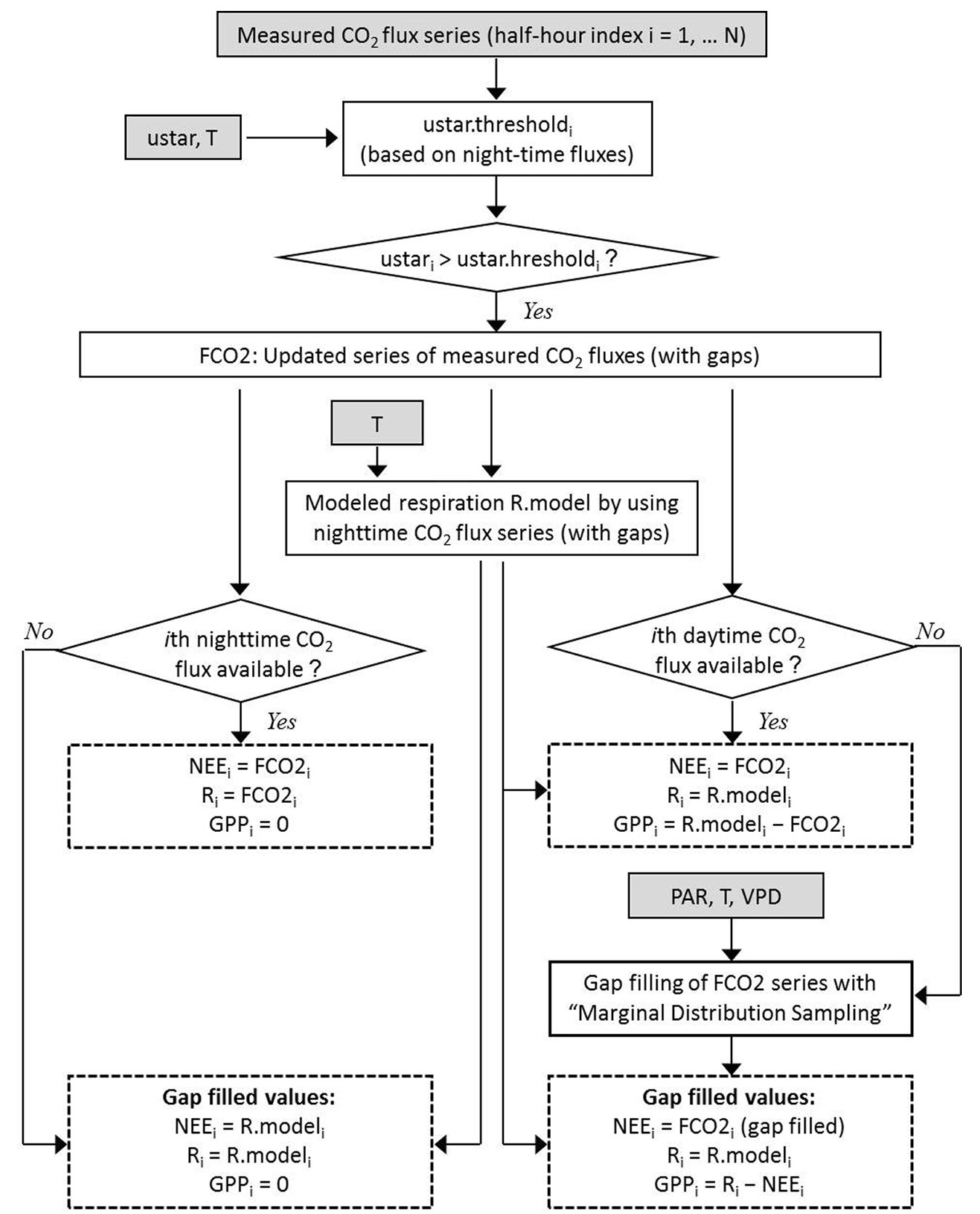
We applied the corrections indicated in Tab. 1, i.e., synchronization between the sonic anemometer and gas analyzer, tilt correction to the vertical velocity measured by the sonic anemometer, conversion of sonic temperature data into air temperature data when needed, and covariance correction for the inclusion of all the frequencies of CO2 turbulent transfer. Raw data were processed and fluxes were calculated using the free software EddyPro (LiCor Biosciences, Lincoln, Nebraska, USA). Outlier cleaning and removal of data below the turbulence threshold were carried out with the free software R (⇒ http://www.r-project.org) and Visual Basic for Application (VBA) within a Microsoft Excel® platform. The procedure to calculate NEE, GPP and respiration using the values measured is depicted in Fig. 1.
Tab. 1 - Corrections applied to raw data recorded by the instruments of the measurement system.
| Problem | Correction method | Bibliographic sources |
|---|---|---|
| Time lag between sonic anemometer and gas analyzer measurement |
Maximization of the covariances between the vertical wind velocity and CO2 and water vapor concentrations | Aubinet et al. ([2]) |
| Sonic anemometer is slightly tilted, requiring correction of wind velocity measurements | Rotation of the coordinate system and re-calculation of horizontal and vertical components of wind velocity | Aubinet et al. ([1]), Wilczak et al. ([45]) |
| Measurement of sonic temperature -instead of air temperature- to calculate the CO2 flux with the equation of Webb et al. ([44]) | Estimation of air temperature and of covariances containing air temperature based on measurements of sonic temperature and air humidity | Schotanus et al. ([39]), Liu et al. ([20]) |
| Missing values of turbulence due to instrumental limitations point out the need of covariance correction | Spectral correction of covariances considering turbulence frequencies that were not captured by the measurement system | Kaimal et al. ([17]), Moore ([28]), Moncrieff et al. ([27]), Massman ([23]), Massman & Clement ([24]) |
Fig. 1 - Scheme of the determination of gap-filled series of Net Ecosystem Exchange (NEE), respiration of the ecosystem (R) and Gross Primary Production (GPP). The input variables are half-hour values of CO2 fluxes, air temperature (T), photosynthetically active radiation (PAR), vapor pressure deficit (VPD) and friction velocity (u star). Gap filling at daytime is carried out by applying “Marginal Distribution Sampling”, which is a methodology proposed by Reichstein et al. ([36]).
We used the model of Hsieh et al. ([15]) to estimate the actual footprint of the measured fluxes. By applying this model, we calculated the distance from the sensors at which footprint contribution is maximum (Hmax) and the surface area including 80% of the footprint value to confirm whether the measured fluxes corresponded to the study area. Ecosystem evapotranspiration was calculated from the latent heat flux λE (in W m-2), following Foken ([11] - eqn. 2):
where λ (≈ 2.454 MJ kg-1) is the latent vaporization heat, which depends slightly on temperature, and E is the water vapor flux (in kg m-2 s-1) corresponding to the evapotranspiration rate, which can be expressed as (eqn. 3):
where ET is the evapotranspiration (in mm H2O d-1), ρH2O is the water density (1025 kg m-3) and Ei is the water vapor flux measured for each of the 48 half-hours in a day.
Removal of CO2 fluxes under low friction velocity conditions and data gap filling
The Eddy covariance technique requires turbulent conditions. The lack of turbulence is associated with low friction velocities (u*). The method described by Reichstein et al. ([36]) was applied to determine the threshold value, using a moving window (± 14 days). During periods when friction velocity (u*) was below a threshold value, CO2 fluxes were removed from the data set. Data gaps were due to technical problems involving sensor calibration, maintenance of the experimental system, power failure and data acquisition failure. Gaps were filled according to the methodology proposed by Falge et al. ([10]) and Reichstein et al. ([36]), and subsequently recommended by Moffat et al. ([26]). The half-hourly Net Ecosystem Exchange was calculated as the sum of CO2 fluxes and expressed on a daily, monthly or annual basis.
The uncertainty in estimates was calculated by applying the method of Hollinger & Richardson ([14]), which is based on the pairwise comparison between CO2 flux values measured within one day under similar meteorological conditions of solar radiation, temperature and wind speed. The gap-filling error was also estimated by first removing each CO2 flux record one at a time from the data set, applying the gap-filling methodology and then comparing the measured and calculated values. This procedure was repeated for each CO2 flux measured, thus obtaining a set of differences between the measured and calculated values. A histogram of these differences can be used to derive the standard deviation of the underlying distribution, in the same way as for the analysis of the random measurement error.
Ecosystem Respiration (Reco) and Gross Primary Production (GPP)
We used an Arrhenius-like model to describe the dependence of respiration on temperature ([21]). Ecosystem Respiration was calculated as follows (eqn. 4):
where Reco is the Ecosystem Respiration (in mg CO2 m-2 s-1), T is the temperature (in °C), Rref is for T = Tref, E0 is a parameter related to activation energy (in °C), Tref is the reference temperature (= 10 °C), and T0 is a parameter set at -46.02 °C.
The methodology described by Reichstein et al. ([36]) was used to determine the values of Rref and E0, based on the regression analysis of fluxes measured during nighttime. A single value was assigned to E0 for the entire study period, while Rref was calculated within a 7-night window. In addition, Reichstein et al. ([36]) provided an equation for estimating the error associated with the calculated Ecosystem Respiration (eqn. 5):
We can now calculate the Gross Primary Production (GPP) as follows (eqn. 6):
A conservative estimate of the error in Gross Primary Production (ΔGPP) is given by (eqn. 7):
Results
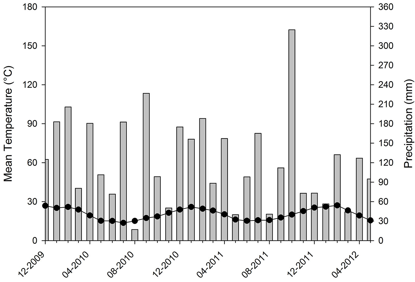
Mean air temperature during the study period ranged between 15.2 °C (June 2011) and 28.3 °C (January 2011). Solar radiation ranged between 32 MJ m-2 in summer and 13 MJ m-2 in winter. Accumulated rainfall for 2010 and 2011 was 1573 mm and 1516 mm, respectively, these values being similar to each other but lower than the climatological mean (Fig. 2).
Fig. 2 - Mean monthly temperature (lines with dots) and monthly accumulated precipitation (bars) during the study period.
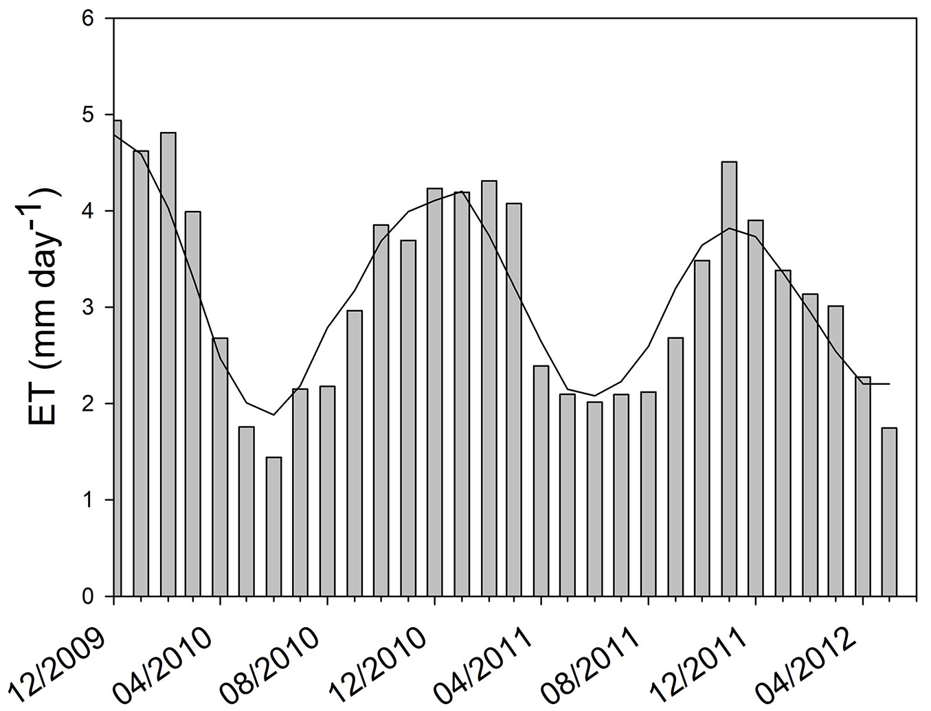
At the beginning of the study period (summer 2009/2010) we obtained the pattern of CO2 flux expected for a green ecosystem. The maximum values of instantaneous CO2 flux to the ecosystem were around -1.8 mg CO2 m-2 s-1 and nighttime respiration reached a peak of 1 mg CO2 m-2 s-1 (Fig. 3). The minimum and maximum values of Ecosystem Evapotranspiration (ET) were obtained in June 2010 (mean daily ET of 1.4 mm) and January 2010 (mean daily ET of about 5 mm), respectively (Fig. 4). Overall, ET was 1161 mm for 2010 and 1132 mm for 2011 (from January to December). By comparing ET and rainfall values, it can be seen that there was a positive water balance (water gain) of 412 mm in 2010 and 384 mm in 2011.
Fig. 3 - Extracts of flux series (January 2010): (a) carbon dioxide, (b) latent heat and (c) sensible heat. The white symbols represent measured fluxes, the black symbols represent gap-filled values.
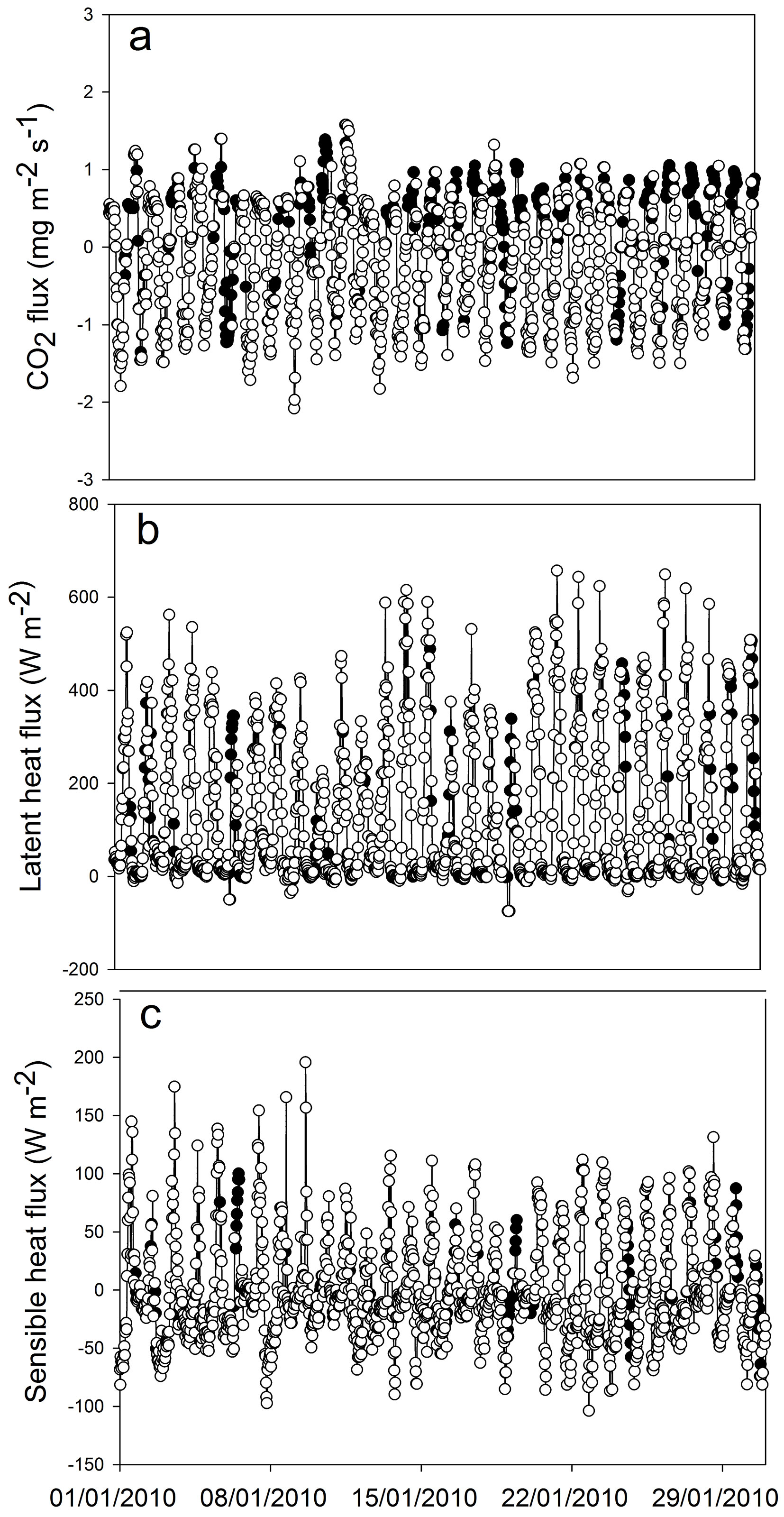
Fig. 4 - Daily mean of evapotranspiration (ET) in mm H2O d-1. The evapotranspiration is calculated by using the latent heat flux measured in the pine forest between December 2009 and May 2012. The moving average line highlights the seasonal behavior of the evapotranspiration.
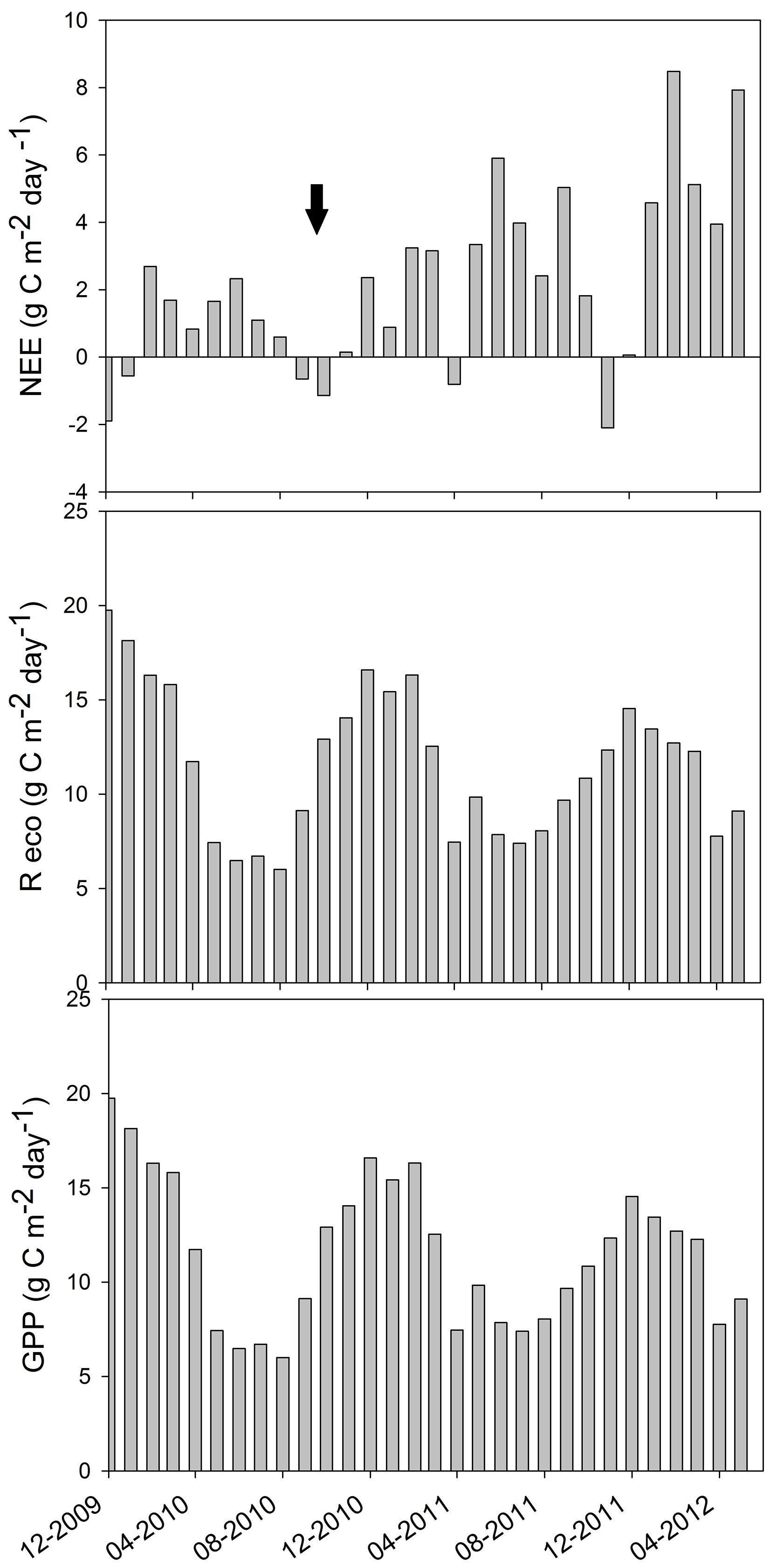
A maximum daily mean NEE of -2.1 g C m-2 d-1 was recorded in November 2011 and a minimum daily mean NEE of 8.5 g C m-2 d-1 in February 2012 (Fig. 5a). The system had positive values of NEE in most of the months (acting as a carbon source), while it had negative values in December 2009, January, September and October 2010, and April and November 2011 (acting as a carbon sink). Ecosystem respiration was calculated with E0 = (344 ± 32) °C, which falls within the range reported by previous studies for other locations ([36]). Ecosystem respiration ranged between 7 and about 20 g C m-2 d-1, with maximum values in summer, as expected based on its dependence with temperature. In general, peaks were observed in February of both years, with only slight differences among the maximum values for the three summers (Fig. 5b). Likewise, highest and lowest values of daily GPP were obtained for the summer and winter months, respectively (Fig. 5c). The maximum GPP was obtained in December 2009, with about 20 g C m-2 d-1, and the minimum GPP was recorded in August 2010, with 6.0 g C m-2 d-1. Maximum GPP decreased from about 20 g C m-2 d-1 in December 2009, to 17 g C m-2 d-1 in December 2010, to 12 g C m-2 d-1 in December 2011. This result is probably due to the growth of the stand, as trees were 6 years old at the beginning of the 2.5-year study period. Mean GPP (± SD) was 4290 ± 473 g C m-2 for 2010 and 4015 ± 485 g C m-2 for 2011. Uncertainty analysis showed a random error of 0.31 mg CO2 m-2 s-1 and the gap-filling error was 0.27 mg CO2 m-2 s-1, resulting in total errors of about 1 g C m-2 d-1.
Fig. 5 - Daily mean of the (a) Net Ecosystem Exchange (NEE), (b) respiration of the ecosystem (Reco) and (c) Gross Primary Production (GPP) of the ecosystem during the measurement period, between December 2009 and May 2012. The moving average of the GPP is also shown, highlighting the seasonal dependence of the pine plantation to carbon storage due to tree growth. Dark arrow points out the sanitary pruning date.
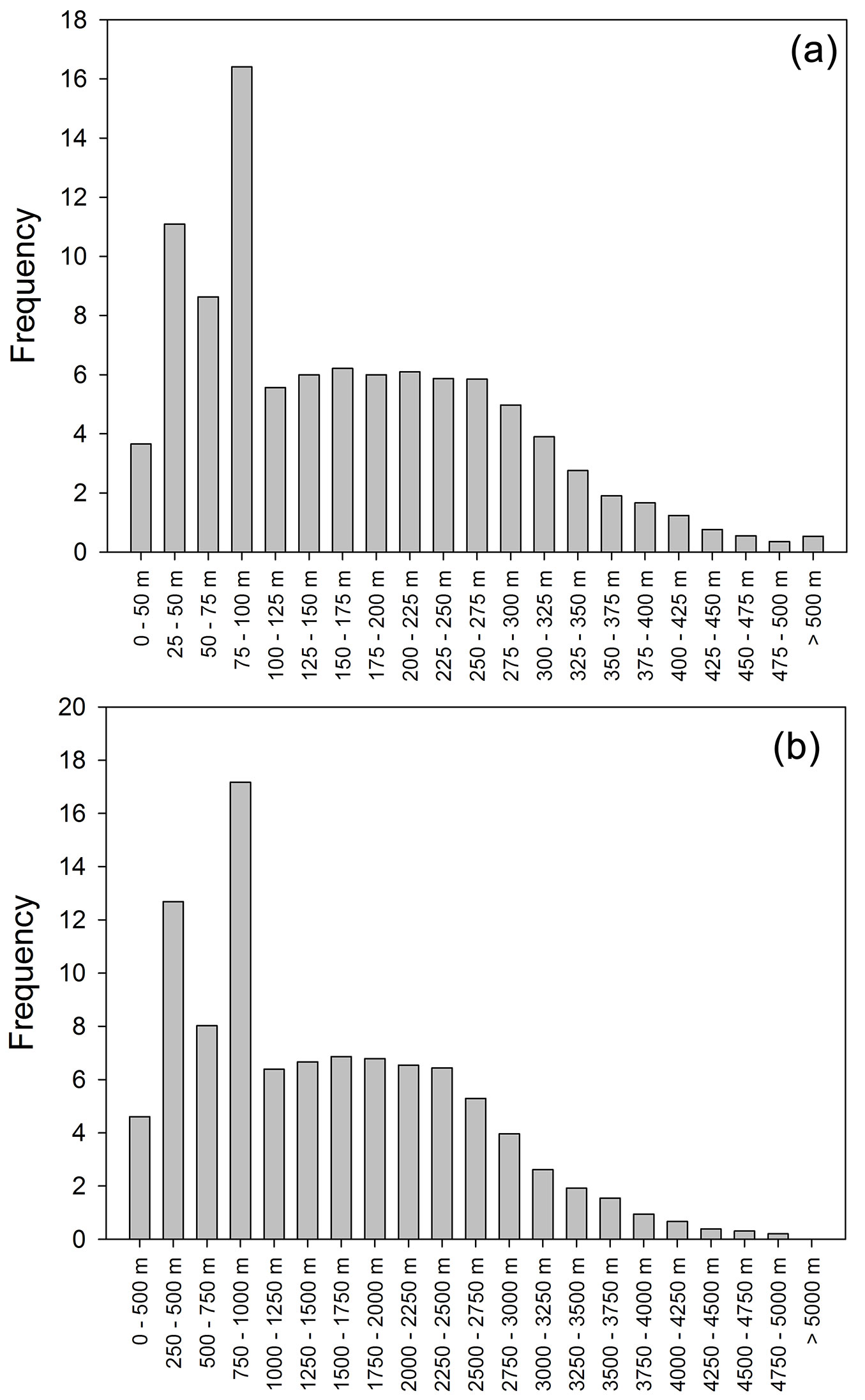
The footprint analysis revealed that the point of maximum contribution of the footprint was at a distance of up to 144 m to the sensors, while 80% of the footprint value was within an area with a radius of 1294 m around the sampling point (Fig. 6). These results confirm that the fluxes measured corresponded to the stands under consideration.
Fig. 6 - Half-hourly frequency (a) of the distance between the flux tower and the footprint maximum and (b) of the distance between the flux tower and the point that represents 80% of the integrated footprint. The footprint calculations were carried out with the footprint model of Hsieh et al. ([15]).
Discussion
The analysis of the GPP dynamics during our 2.5-year study shows maximum values in the summer months, mainly December. The highest instantaneous rates ranged between -2.5 and -3.0 mg CO2 m-2 s-1, these values being similar to those reported for other areas. For example, Goldstein et al. ([12]) obtained GPP values ranging between 3.3 and 4.0 mg CO2 m-2 s-1 for young ponderosa pine plantations in the Sierra Nevada Mountains, California. On the other hand, Coursolle et al. ([7]) reported maximum NEE values of up to -2.0 mg CO2 m-2 s-1 for conifer stands of different age, while young forest stands had a remarkably lower NEE (about -0.25 mg de CO2 m-2 s-1).
Net carbon gain is expected to occur in a forest, as reported for other forests of the world ([9], [22]). Many studies have recorded an increase in CO2 emissions after harvest without providing any information on their origin, while others found no effect. Covington ([8]) and Yanai et al. ([46]) estimated a carbon loss of 20% following tree harvest. Pruned branches left on the forest floor can be expected to contribute to soil carbon, but only as long as carbon fixation rate exceeds their respiration rate. Often, changes in temperature and humidity due to land work lead to changes in ecosystem respiration rates ([42], [46], [13]).
However, some studies have also reported positive NEE values but the system acted as a net carbon source. For example, Cai et al. ([5]), who studied a hybrid poplar plantation on a former agricultural land in Alberta, Canada, found that the annual carbon balance shifted from a net source of 312 g C m-2 in year 1, to approximately C-neutral in year 5. Law et al. ([19]) stated that ecosystem respiration in young stands may be higher than the NPP of the regrowth due to the decomposition of dead biomass from the previous forest generation. They compared net ecosystem production (NEP) between young (14 years old) and old (45/250 years old) pine stands in Oregon and found that the old stands gained carbon at a rate of 28 g C m-2 yr-1, while the young stands lost carbon at a rate of 32 g C m-2 yr-1. This indicates that the young stands did not yet reach the net sequestration capacity of the old ones. Our study area also experienced a drastic ecosystem alteration because the original ecosystem (natural grassland) was replaced by a plantation in 2003. We detected that the system acted as a carbon sink only during December 2009, January, September and October 2010, and April and November 2011.
It is probably that the high ecosystem respiration rates obtained in the study area resulted from pruning conducted prior to our measurements and from the sanitary pruning made during the course of this study in October 2010, after which a large amount of cut branches accumulated on the ground until they were subjected to decomposition, whose rate is expected to increase with time. It is reasonable to suppose that the remains of branches left on the ground increased the amount of soil carbon available for the ecosystem respiration. Noormets et al. ([31]) found that respiration of plant litter lasted for 2 years, while heterotrophic respiration (from root remains) showed an emission peak at 3 and 4 years after harvest. In addition, they stated that part of the “old” soil carbon pool was respired, and that it took 4.5 years for the plantation to act as a carbon sink and 9.5 years to regain the carbon sink capacity after harvest.
Forestry also has a substantial impact on the albedo and the hydrological balance, in terms of evapotranspiration, water infiltration into the soil and water lost by runoff. These factors, which may account for major changes in local climate conditions and water availability downstream ([4], [32]), should be taken into account when planning a major land-use change such as the one considered in our study, i.e., from grassland to plantation. In the study area, the dynamics of the river basin appears to be unaffected by forest stands because water is not a limiting resource.
Conclusions
In our study area, the estimated respiration rates resulted from the respiration of trees, soil microorganisms and soil carbon. The replacement of the original grassland by a pine plantation (e.g., removal of the original vegetation, land preparation) led to changes with long-term consequences. A large amount of cut branches resulting from pruning activities were accumulated on the ground and subjected to decomposition. As a consequence, the studied forest had high ecosystem respiration rates, up to 20 g C m-2 d-1 in summer. The decrease in GPP with time and the maintenance of ecosystem respiration rates cause NEE to increase with time, with positive values indicating carbon loss. Thus, the system acted as a carbon source in most of the months, in contrast to that expected for a forest system.
Acknowledgements
Thanks are due to Forestal Bosques del Plata S.A. (FBP) for allowing field measurements in the plantation (Technical Cooperation Agreement INTA/FBP No. 20020); to Cesar Niklas, German Becerro and Darío Britez from FBP for their assistance with the logistics; to Mr. Fabián, the operator of the fire surveillance tower; to Martin Bellomo and Jorgelina Corin for their help in sensor setting-up and maintenance. Silvia Pietroskovsky improved the English version. NL and PC are PhD fellows of the Consejo Nacional de Investigaciones Cientificas y Ténicas (CONICET), Argentina, and KR was supported by the Center for International Migration (CIM), Frankfurt, Germany. This work was supported by the Instituto Nacional de Tecnología Agropecuaria (INTA), Projects AERN 3632, AERN 239321 and PNNAT 1128023.
References
CrossRef | Gscholar
CrossRef | Gscholar
CrossRef | Gscholar
CrossRef | Gscholar
Gscholar
CrossRef | Gscholar
Gscholar
CrossRef | Gscholar
CrossRef | Gscholar
CrossRef | Gscholar
Authors’ Info
Authors’ Affiliation
Nuria Lewczuk
Klaus Richter
INTA - Instituto de Clima y Agua, N. Repetto y De Los Reseros s/n, 1686 Hurlingham, Provincia de Buenos Aires (Argentina)
Departamento de Ecología, Genética y Evolución, Instituto IEGEBA (CONICET-UBA), Facultad de Ciencias Exactas y Naturales, Universidad de Buenos Aires (Argentina)
Corresponding author
Paper Info
Citation
Posse G, Lewczuk N, Richter K, Cristiano P (2016). Carbon and water vapor balance in a subtropical pine plantation. iForest 9: 736-742. - doi: 10.3832/ifor1815-009
Academic Editor
Tamir Klein
Paper history
Received: Aug 18, 2015
Accepted: Jan 28, 2016
First online: May 25, 2016
Publication Date: Oct 13, 2016
Publication Time: 3.93 months
Copyright Information
© SISEF - The Italian Society of Silviculture and Forest Ecology 2016
Open Access
This article is distributed under the terms of the Creative Commons Attribution-Non Commercial 4.0 International (https://creativecommons.org/licenses/by-nc/4.0/), which permits unrestricted use, distribution, and reproduction in any medium, provided you give appropriate credit to the original author(s) and the source, provide a link to the Creative Commons license, and indicate if changes were made.

Web Metrics
Breakdown by View Type
Article Usage
Total Article Views: 50524
(from publication date up to now)
Breakdown by View Type
HTML Page Views: 41957
Abstract Page Views: 3560
PDF Downloads: 3580
Citation/Reference Downloads: 85
XML Downloads: 1342
Web Metrics
Days since publication: 3463
Overall contacts: 50524
Avg. contacts per week: 102.13
Article Citations
Article citations are based on data periodically collected from the Clarivate Web of Science web site
(last update: Mar 2025)
Total number of cites (since 2016): 13
Average cites per year: 1.30
Publication Metrics
by Dimensions ©
Articles citing this article
List of the papers citing this article based on CrossRef Cited-by.
Related Contents
iForest Similar Articles
Research Articles
Soil respiration and carbon balance in a Moso bamboo (Phyllostachys heterocycla (Carr.) Mitford cv. Pubescens) forest in subtropical China
vol. 8, pp. 606-614 (online: 02 February 2015)
Technical Notes
The impact of pruning on tree development in poplar Populus × canadensis “I-214” plantations
vol. 15, pp. 33-37 (online: 30 January 2022)
Research Articles
Day and night respiration of three tree species in a temperate forest of northeastern China
vol. 8, pp. 25-32 (online: 26 May 2014)
Research Articles
Links between phenology and ecophysiology in a European beech forest
vol. 8, pp. 438-447 (online: 15 December 2014)
Research Articles
Carbon storage and soil property changes following afforestation in mountain ecosystems of the Western Rhodopes, Bulgaria
vol. 9, pp. 626-634 (online: 06 May 2016)
Research Articles
Multi-temporal influence of vegetation on soil respiration in a drought-affected forest
vol. 11, pp. 189-198 (online: 01 March 2018)
Research Articles
Effects of thinning and pruning on stem and crown characteristics of radiata pine (Pinus radiata D. Don)
vol. 10, pp. 383-390 (online: 16 March 2017)
Research Articles
Thinning effects on soil and microbial respiration in a coppice-originated Carpinus betulus L. stand in Turkey
vol. 9, pp. 783-790 (online: 29 May 2016)
Review Papers
Separating soil respiration components with stable isotopes: natural abundance and labelling approaches
vol. 3, pp. 92-94 (online: 15 July 2010)
Short Communications
Influences of Black Locust (Robinia pseudoacacia L.) afforestation on soil microbial biomass and activity
vol. 9, pp. 171-177 (online: 16 February 2015)
iForest Database Search
Search By Author
Search By Keyword
Google Scholar Search
Citing Articles
Search By Author
Search By Keywords
PubMed Search
Search By Author
Search By Keyword


