Modelling diameter distribution of Tetraclinis articulata in Tunisia using normal and Weibull distributions with parameters depending on stand variables
iForest - Biogeosciences and Forestry, Volume 9, Issue 5, Pages 702-709 (2016)
doi: https://doi.org/10.3832/ifor1688-008
Published: May 17, 2016 - Copyright © 2016 SISEF
Research Articles
Abstract
The objective of this study was to evaluate the effectiveness of both Normal and two-parameter Weibull distributions in describing diameter distribution of Tetraclinis articulata stands in north-east Tunisia. The parameters of the Weibull function were estimated using the moments method and maximum likelihood approaches. The data used in this study came from temporary plots. The three diameter distribution models were compared firstly by estimating the parameters of the distribution directly from individual tree measurements taken in each plot (parameter estimation method), and secondly by predicting the same parameters from stand variables (parameter prediction method). The comparison was based on bias, mean absolute error, mean square error and the Reynolds’ index error (as a percentage). On the basis of the parameter estimation method, the Normal distribution gave slightly better results, whereas the Weibull distribution with the maximum likelihood approach gave the best results for the parameter prediction method. Hence, in the latter case, the Weibull distribution with the maximum likelihood approach appears to be the most suitable to estimate the parameters for reducing the different comparison criteria for the distribution of trees by diameter class in Tetraclinis articulata forests in Tunisia.
Keywords
Diameter Class Model, Normal Distribution, Weibull Distribution, Maximum Likelihood Approach, Moments Method, Tetraclinis articulata
Introduction
Thuya (Tetraclinis articulata [Vahl.] Mast.) is a semiarid Mediterranean forest species which extends discontinuously from North Africa to south-western Europe. The natural character and the limited geographic distribution area of the species make it of particular ecological interest in terms of biodiversity conservation. Thuya forests provide highly valuable services such as soil erosion control, biodiversity conservation and CO2 fixation, and are suitable for afforestation programs in arid or semiarid environments, where few species are able to grow ([48]), and areas with severely eroded soils ([19]).
In addition, these stands are of potential economic and social interest for the rural populations, not only in Tunisia where they cover 33000 ha ([16]), but also in Algeria and Morocco, covering more than 1000000 ha in Maghreb ([12]). Thuya timber is widely used in construction, handicraft and cabinetmaking due to its hardness, veneer, durability and fragrance. A secondary traditional use of this species is resin production to obtain sandarac gum. However, overexploitation for timber, irrational resin tapping, grazing pressure and uncontrolled fires have resulted in highly degraded forests ([12], [18]). The extinction of this species has only been avoided by its resprouting capacity. The current degraded state has left these forests devoid of large trees, so the main production presently comprises small pieces of wood for fuel and fencing ([17]). However, the profitability of these forests could be improved by exploiting other uses of the wood such as in industry, production of decorative objects, etc.
Improving the profitability of wood and resin production, along with the need to preserve and improve Tunisian thuya stands, which play a key ecological role in arid or semiarid environments, necessitates the development of models for quantitatively assessing the production of wood at different forest sites and under different management schedules to ensure a sustained yield. A first step towards this objective was the development of tree-level models relating common variables measured during forest inventories, such as breast height diameter, with relevant tree attributes like total tree height, crown diameter, height to crown base, stem taper curve and tree volume ([8]). The diameter-growth dynamics of the trees was studied by developing a distance-independent individual tree diameter increment model ([46]). A stand-level growth and yield model has recently been developed consisting of a site index sub-model and a system of compatible stand attribute equations presented in the form of a stand density management diagram ([47]). The next step would be to characterize the stand diameter structure.
Fonseca et al. ([21]) state that detailed information on the variability of tree diameters in natural and altered stands is key to sustainable forest management and is needed to assess carbon sequestration in forest ecosystems. Tree diameter distributions play an important role in stand management. For example, data regarding the number of trees per diameter class in a stand where a given silvicultural treatment has been applied are of particular interest because the diameter size will determine the industrial use of the wood and thus the price of the different products ([24]). Diameter distribution data at stand level also provides a more scientific basis for forest managers to choose which trees should be harvested ([45]).
Different types of parametric density functions have been used to describe tree diameter distribution in forest stands, including the Normal ([37]), Log-normal ([5], [37]), Gamma ([39]), Beta ([13], [42]), Johnson’s SB ([27], [42], [21]) and the Weibull distribution ([2], [42]). Mateus & Tomé ([33]) used Johnson’s distribution for modeling the diameter distribution of first-rotation eucalyptus plantations in Portugal. Gorgoso et al. ([25]) compared the accuracy of the Weibull, Johnson’s SB and beta distributions for modeling even-aged stands of Pinus pinaster Ait., Pinus radiata D. Don and Pinus sylvestris L. in northwest Spain, and Binoti et al. ([4]) evaluated the effectiveness of fatigue life, Frechet, Gamma, Generalized Gamma, Generalized Logistic, Log-logistic, Nakagami, Beta, Burr, Dagum, Weibull and Hyperbolic distributions for describing diameter distribution Tectona grandis L. stands subjected to thinning treatments at different ages in Brazil. Sghaier & Palm ([45]) used Pearson’s type I function for modeling diameter distribution of Pinus halepensis Mill. stands in Tunisia.
The objective of this study is to model the diameter distribution of the main Tetraclinis articulata stands in Tunisia. To achieve this objective, we compared the Normal distribution, given its ease of use, and the two-parameter Weibull distribution, since it has been shown to be the most suitable in many cases ([7], [34]).
Material and ethods
Study area and data collected
The natural Tetraclinis articulata stands at Jbel Lattrech forest in north-eastern Tunisia cover an area of approximately 4.000 hectares and are essentially mono specific and homogeneous. The climate is semi-arid, with an annual average precipitation of 393 mm, of which 95 % of rain falls between September and May. The average minimum temperatures for the coldest month (January) and maximum for the hottest month (August) are 8.4 and 30.5 °C, respectively ([3]). The study zone is located on Oligocene sandstones where there are groupings of Tetraclinis articulata - Lavandula stoechas, dominated by Cistus monspelliensis L., Genista aspalathoides Lam., Erica arborea L., Brachypodium ramosum Roemer et Schultes, Avena bromoides Gouan and Lupinis angustifolius L. ([36]).
The data used to develop the diameter distribution model were collected in 2009 from 50 temporary circular sample plots of variable radius and established such that they cover a wide range of age, density and site quality combinations. The size of the plots ranged from 88 to 835 m2, depending on the stand density, so as to include at least 40 measured trees per plot. The diameter at breast height of all trees in each plot (down to a minimum diameter of 5 cm) was measured to the nearest 0.1 cm. Additionally, the heights of a random sample of 11 trees per plot (including the 4 largest trees) were measured to estimate mean height. Dominant height was calculated from the four largest trees per plot, and age was estimated from stem analysis on fallen trees by counting the number of rings at 0.30 m (see [8] for more details on data collection). Tab. 1 shows the main stand variables measured in the 50 plots.
Tab. 1 - Summary of main stand variables for the sample used for modelling ([47]).
| Variables | Mean | STD | Min | Max |
|---|---|---|---|---|
| Density (stems ha-1) | 1860 | 865 | 479 | 4533 |
| Age (years) | 57 | 10 | 36 | 77 |
| Site index (m) | 5.06 | 1.08 | 2.83 | 7.78 |
| Basal area (m2 ha-1) | 12.90 | 6.39 | 2.32 | 27.74 |
| Quadratic mean diameter (cm) | 9.41 | 1.55 | 6.32 | 12.95 |
| Dominant diameter (cm) | 12.76 | 2.32 | 7.85 | 17.43 |
| Dominant height (m) | 6.52 | 1.38 | 4.20 | 11.00 |
| Mean height (m) | 5.46 | 1.09 | 3.61 | 9.17 |
| Volume (m3 ha-1) | 36.14 | 22.13 | 5.16 | 111.61 |
Diameter distribution unctions
We tested two distribution functions: the Normal function, known for its ease of use ([29]), and the Weibull function, most frequently used because of its flexibility, simplicity and existence of a closed form solution for its CDF ([10], [35], [41], [24]).
Normal distribution
The equation for the normal probability density function is (eqn. 1):
where x is the random variable, and m and σ are its arithmetic mean and standard deviation, respectively.
The cumulative probability distribution of the normal function is (eqn. 2):
The two parameters which define the normal distribution (arithmetic mean and the standard deviation) can be estimated by using the following expressions ([15] - eqn. 3, eqn. 4):
where n indicates the number of trees per plot and xi (cm) the diameter at breast height of each tree.
Weibull distribution
The variety of shapes that can be taken by the Weibull distribution makes it particularly suitable for representing tree diameter distribution. The equation for the Weibull probability density function is as follows (eqn. 5):
for x ≥ a, a ≥ 0, b > 0, c > 0 or 0 if not. The cumulative probability distribution of the Weibull function is (eqn. 6):
for x > a. This function is defined by three parameters: a is the location parameter, b is the scale parameter and c is the shape parameter.
Parameter a, commonly termed the location parameter, identifies the lower bound of the diameter distribution. For fixed values of b and c, changes in the parameter a simply shift the entire distribution along the x-axis. Parameter b is the scale parameter, and point x = a + b corresponds approximately to the 63rd percentile of the distribution. Parameter c defines the shape of the Weibull distribution. When c < 1, the distribution has a reverse-J shape. In the special case where c = 1, the Weibull distribution is reduced to the exponential distribution. When c > 1, the distribution is mound-shaped, approximately equivalent to the Normal distribution for c = 3.6. When c is between 1 and 3.6 the Weibull distribution is positively skewed, and is negatively skewed when c is greater than 3.6 ([2]).
The most frequently used methods to estimate the parameters of the Weibull distribution, are the maximum likelihood method ([28]) and the method of moments ([6]). Parameter a can be considered the smallest possible diameter in the stand and thus should be between zero and the minimum observed value in some cases ([2]). In some studies, the parameter a is arbitrarily fixed at 0.5 dmin ([30]) or at zero ([24], [44]), thus reducing the function to a two-parameter Weibull distribution which is easier to model and provides similar results to those of the three-parameter Weibull function, at least for even-aged, single-species stands ([34], [32]).
The two-parameter Weibull function (with the location parameter a = 0) was considered in this study as follows (eqn. 7):
where x is the random variable, b the scale parameter and c the shape parameter that controls the skewness.
Maximum likelihood estimator (MLE)
The maximum likelihood method is a commonly used procedure for the Weibull distribution in forestry because it has certain desirable properties ([30]). Estimation of the parameters using maximum likelihood has been found to produce consistently better goodness-of-fit statistics compared to other methods, but it also puts the greatest demands on the computational resources ([11]). If we consider the Weibull probability density function given in eqn. 7, then the likelihood function (L) will be (eqn. 8):
Taking the logarithms from eqn. 8, differentiating with respect to b and c respectively, and satisfying the following equations ([14], [38], [20] - eqn. 9, eqn. 10):
where n equals the number of sample observations in a Weibull distribution and xi the diameter of each tree. The value of c must be obtained from eqn. 9 by using standard iterative procedures and then it is used in eqn. 10 to obtain b.
Method of moments (MOM)
The method of moments is another technique commonly used for parameter estimation. In the Weibull distribution, the k moment readily follows from eqn. 7 and is ([30] - eqn. 11):
where Γ (Gamma function) is Γ(s) = ∫ xs-1 e-x dx (s>0). Then from eqn. 11, we can find the first and the second moment as follows (eqn. 12, eqn. 13):
which gives (eqn. 14):
where σ2 is the variance of tree diameters in a plot, and m1, m2 are the arithmetic and quadratic mean diameter in a plot, respectively.
When σ2 is divided by the square of m1, the expression for obtaining c is (eqn. 15):
In order to estimate b and c, we need to calculate the arithmetic mean diameter d and the variance σ2 of the observed distribution and obtain the estimator of c in eqn. 15. eqn. 15 was resolved by an iterative procedure. When the value of the location parameter (a) is zero, the scale parameter (b) can then be calculated directly using the following equation ([24], [44] - eqn. 16):
where d is the arithmetic mean diameter.
Method comparison
To determine whether the adjusted theoretical distribution provides a good representation of what is observed, we used the chi-square test (χ2). This test requires some extreme classes to be grouped when there are an insufficient number of observations ([15]). For this reason, the following goodness-of-fit statistics were computed for each method: the mean bias, which reflects the deviation of the model with respect to observed values and the root mean-square error (RMSE), which is a measure of the precision of the estimates.
For the calculation of these statistics, the observed value Yi and the theoretical value Yi were calculated for each diameter class per plot (2 cm diameter class). In addition, the error index ([43]) was calculated (eqn. 17):
where Yi and Yi are the observed and predicted number of trees in diameter class k for the i-th plot. The sum includes all diameter classes in the i-th plot. In this error index, we can multiply the absolute difference between the observed and predicted number of trees per diameter class by the volume, using an equation developed by Sghaier et al. ([47]): v = 2.182 · 10-2 · d2.89, R2 = 0.917. The diameter used in this equation corresponds to the middle diameter class. In this case (eqn. 18):
This index can also be expressed relatively as a percentage by dividing it by the total volume of the observed distribution in the plot ([29] - eqn. 19).
The latter error index was systematically calculated for each plot in this study.
Parameter prediction: distribution parameters with stand variables
In order to predict the parameters of the distribution functions directly from the stand variables using simple regression models, correlation analyses were carried out by estimating Pearson’s correlation coefficients between the estimated parameters corresponding to each plot and different stand variables. The stand variables chosen were: age (A), density (N), dominant height (Hd), mean height (Hm), quadratic mean diameter (dg), arithmetic mean diameter (d), 25% percentile (P25), median (P50), 75% percentile (P75) of the stand, and natural logarithm transformations for the quotient of the 25% percentile, the 50% percentile, the 75% percentile and the mean diameter by the quadratic mean diameter (LP25, LP50, LP75, and Ld, respectively).
To predict the fitting parameters from the yield table using the Normal and Weibull distribution, the mean diameter and the variance must be known (first and second order moments of the distribution, respectively). The variance can be directly obtained from the arithmetic and the quadratic mean diameter ([22]) by the following expression (eqn. 20):
The mean diameter can be modeled with eqn. 21, which ensures the prediction of dÌis lower than the quadratic mean diameter (dg - eqn. 21):
where X is a vector of independent stand variables in a fixed instant and β is the vector of parameters to be estimated ([24], [44]).
To select the model, the bias, the mean square error and the adjusted determination coefficient were computed.
Results
Tab. 2 shows summary descriptive statistics for the estimated parameters.
Tab. 2 - Summary statistics of the estimated parameters for the studied distributions (50 plots). (Sigma): σ; (predicted mean): μ.
| Distribution | Method | Parameter | Mean | Minimum | Maximum | CV% |
|---|---|---|---|---|---|---|
| Weibull | MLE |
b
|
10.01 | 6.680 | 13.794 | 16.5 |
c
|
4.134 | 3.137 | 7.087 | 18.6 | ||
| MOM |
b
|
9.986 | 6.657 | 13.777 | 16.6 | |
c
|
4.418 | 3.077 | 7.410 | 20.8 | ||
| Normal | - | Predicted mean | 9.087 | 6.240 | 12.550 | 16.1 |
| Sigma | 2.427 | 1.011 | 3.862 | 26.3 |
In order to adjust the models to predict the parameters of the theoretical distributions using the stand variables, Pearson’s linear correlations for estimated parameters were calculated (Tab. 3).
Tab. 3 - Correlations between stand variables and parameters estimated with the three studied distributions. (***): P<0.001; (**): P<0.01; (*) P<0.05; (A): age (years); N: density (trees ha-1); Hd: dominant height (m); Hm: mean height (m); dg: quadratic mean diameter (cm); (dÌ ): mean diameter (cm); P25: 25% percentile (cm); P50: 50% percentile (cm); P75: 75% percentile (cm); LP25: ln(P25/dg); LP50: ln(P50/dg); LP75: ln(P75/dg); Ld=ln(d/dg); ln: natural logarithm.
| Variable | Normal distribution | Weibull distribution | |||
|---|---|---|---|---|---|
| Maximum Likelihood | Moments | ||||
| b | c | b | c | ||
| A | 0.088 | 0.218 | 0.176 | 0.221 | 0.110 |
| N | -0.054 | -0.170 | -0.066 | -0.174 | -0.081 |
| H d | 0.665*** | 0.667*** | -0.368** | 0.670*** | -0.464*** |
| H m | 0.720*** | 0.762*** | -0.335* | 0.763*** | -0.456*** |
| d g | 0.872*** | 0.999*** | -0.380** | 0.999*** | -0.511*** |
d
|
0.844*** | 0.998*** | -0.336* | 0.998*** | -0.469** |
| P 25 | 0.648*** | 0.923*** | -0.109 | 0.923*** | -0.226 |
| P 50 | 0.768*** | 0.970*** | -0.231 | 0.971*** | -0.367** |
| P 75 | 0.857*** | 0.976*** | -0.359* | 0.976*** | -0.505*** |
| LP 25 | -0.617*** | -0.253 | 0.742*** | -0.254 | 0.783*** |
| LP 50 | -0.370** | -0.064 | 0.602*** | -0.061 | 0.582*** |
| LP 75 | 0.203 | 0.203 | -0.042 | 0.206 | -0.155 |
| Ld | -0.811*** | -0.463*** | 0.884*** | -0.459*** | 0.908*** |
The highest Pearson correlation between the parameters of Normal and Weibull distribution and the stand variables was obtained with dg and its natural logarithm transformations. The values obtained for Pearson’s linear correlation between the Ld parameter and the two estimated parameters of the Weibull distribution using the Maximum Likelihood and moments approaches were -0.463 and -0.459 for parameter b and 0.884 and 0.908 for parameter c. In the case of the shape parameter (c), the highest values obtained for Pearson’s linear correlation were for the variable Ld (Tab. 3). The values obtained for the coefficients of determination were 91% and 96% for models that relate the parameter c to the variable Ld (Tab. S1 in Appendix 1).
As regards the variance of the Normal distribution and the scale parameter (b) for the Weibull distribution, the results also show good linear relationships between these parameters and the measured stand variables. It appears that there is a logarithmic relation between the variance and quadratic mean diameter (dg). The coefficient of determination was 78% (Tab. S1 in Appendix 1).
Note that the mean diameter is needed to estimate the shape parameter (c) in both parameter prediction methods of the Weibull distribution as well as in the Normal distribution. Since the yield tables generally only give the quadratic mean diameter (dg), an equation was employed to predict the mean diameter from the quadratic mean diameter (dg), the mean height (Hm) and the age (A) of the stand (Tab. S2 in Appendix 1).
According to the fitted prediction equation of the mean diameter (Tab. S2 in Appendix 1), the mean quadratic diameter (dg), the mean height (Hm) and the age of the stand (A) must be known. Of these three parameters, only the mean height (Hm) cannot be directly obtained from yield tables and was therefore estimated by the fitting equation (eqn. 22) using the dominant height (Hd) disaggregated from yield tables as an independent variable (eqn. 22):
with R2 = 0.989 and CV% = 11.03. The expected theoretical values for each plot are calculated using the three studied distributions with the two parameter prediction methods (estimated and prediction parameters). The observed, estimated and predicted values were grouped for each plot in 2 cm diameter classes. The results of the different comparison criteria are shown in Tab. 4.
Tab. 4 - Bias, mean absolute error, residual mean square error and mean error index in number of trees for the three compared distributions (Weibull MLE, Weibull MOM and Normal) and the two methods of construction (parameter estimation and parameter prediction).
| Methods | Comparison criteria | Weibull | Normal | |
|---|---|---|---|---|
| Maximum Likelihood |
Moments | |||
| Parameters estimation | Bias | 0.0097 | 0.0068 | 0.0185 |
| MAE | 1.7140 | 1.7145 | 1.6197 | |
| RMSE | 5.2173 | 5.3054 | 4.7749 | |
EI’ % |
32.61 | 33.40 | 31.42 | |
| Parameters prediction | Bias | 0.0164 | 0.0063 | 0.0220 |
| MAE | 1.7180 | 1.7592 | 1.8958 | |
| RMSE | 5.3606 | 5.6220 | 6.1839 | |
EI’ % |
32.25 | 34.03 | 35.13 | |
In the parameter estimation, the Normal distribution is the most suitable for all the comparison criteria evaluated, with the exception of bias. Furthermore, the two parameter estimation approaches of the Weibull function gave similar results, although the maximum likelihood approach (MLE) was found to be slightly better.
In contrast to the parameter prediction in the first model construction approach (parameter estimation), the results obtained for parameter prediction revealed that the Weibull distribution was better for all the comparison criteria used. In this case, the maximum likelihood method also provided the best results, with the exception of the bias, for which the method of moments gave the lowest value.
In addition to comparing the distributions according to the Reynolds’ index error (EI %), which is calculated for each plot, an analysis of variance (ANOVA) was performed for each model construction method. The results obtained reveal that there is no significant difference between the three distributions in each of the two model construction methods (α = 0.75 for parameter estimation and α = 0.57 for parameter prediction, respectively).
The Weibull distribution, using the method of moments, occupied the same intermediate position with the exception of the bias, for which it gave the lowest value in both cases (estimated and prediction parameters). To analyze these results in greater depth, some additional graphs were produced. The first two, (Fig. 1 and Fig. 2), present the values of Bias and RMSE in each diameter class. Fig. 3 shows the mean value of the error index (EI %) in each density class.
Fig. 1 - Values of bias in number of trees in each diameter class obtained using two fitting methods of the two-parameter Weibull distribution and Normal distribution. (a) Parameter estimation; (b): parameter prediction.
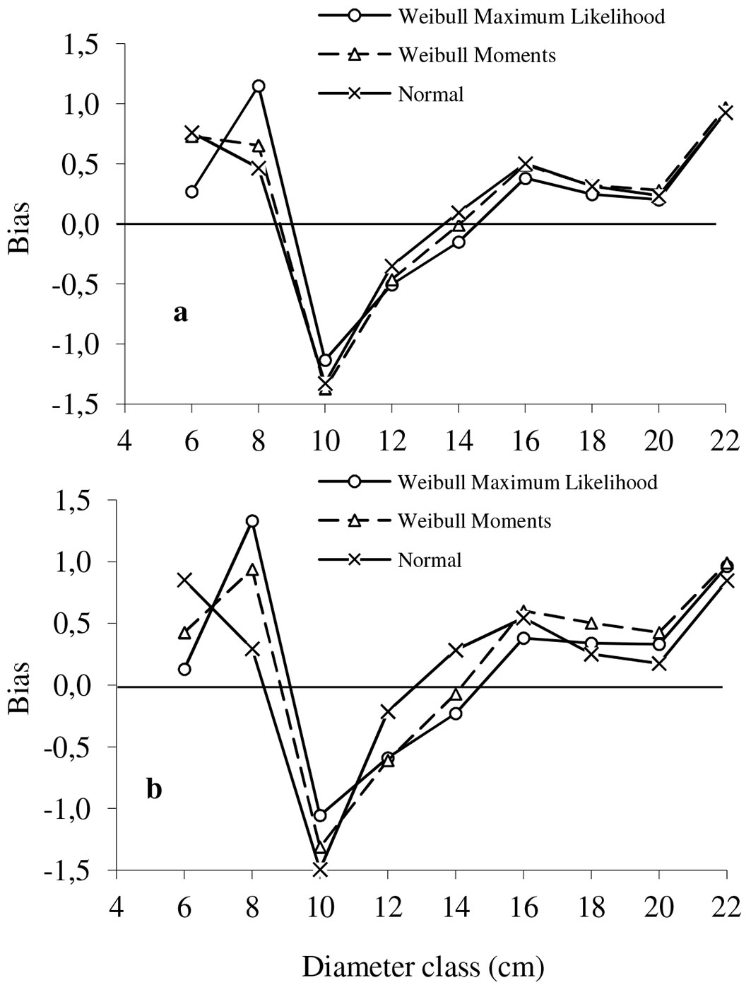
Fig. 2 - Values of mean square error (RMSE) in number of trees for each diameter class obtained using the two fitting methods of the two-parameter Weibull distribution and Normal distribution. (a) Parameter estimation; (b) parameter prediction.
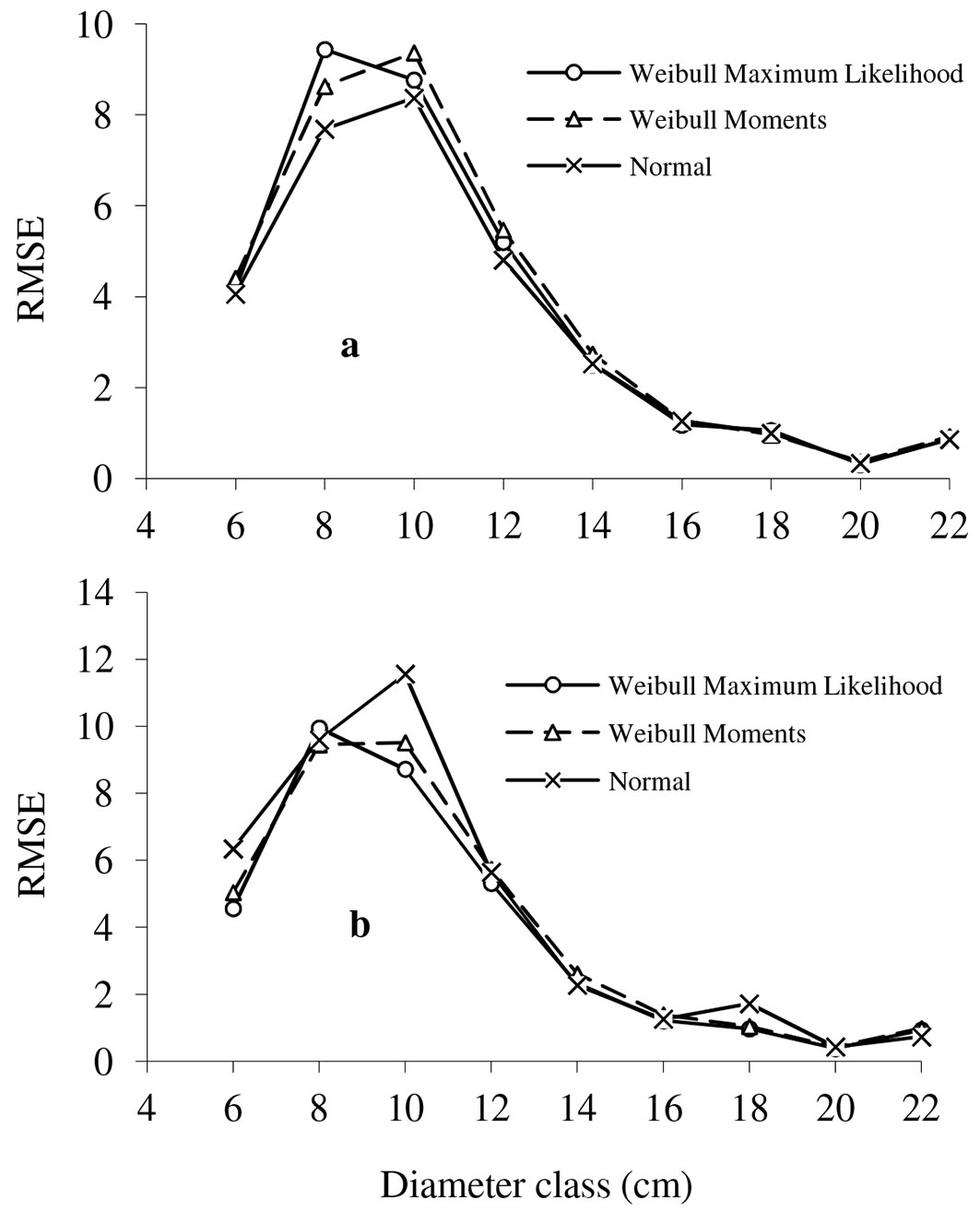
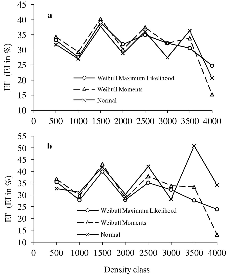
Fig. 3 - Mean value of error index EI % in each density class (trees ha-1). (a) Parameter estimation; (b) parameter prediction.
According to the values for bias (Fig. 1), all the distributions underestimated the frequency of trees in the smallest and largest diameter classes, and overestimated them for the 10 cm diameter class under both parameter construction methods. With the exception of the 8 cm diameter class, for which the Weibull maximum likelihood method gives the highest value, the distributions compared present a similar level of precision, though the Normal distribution is slightly better, especially for parameter prediction.
As regards the mean square error (Fig. 2), although there are slight differences in the smallest diameter classes (lower or equal to 10 cm), the distributions gave similar results for diameter classes of 12 cm and above, being the Weibull distributions slightly superior in the case of parameter prediction.
For the Reynolds error index (EI %), Fig. 3 shows the variation of the mean value of this criterion according to stand density class (trees ha-1). For both model construction approaches, the Weibull distribution, using the maximum likelihood method to estimate the parameters, appears to give the most stable results of the three studied methods. In addition to its stability across all the density classes, this method also provides the most accurate results for the parameter prediction approach (Fig. 3).
According to the distribution of trees per diameter class in each of the 50 measured plots, three types of distribution shape were observed (symmetric distribution, right dissymmetric distribution and reverse-J distribution). In order to better appreciate the capacity of the adjusted models to predict the number of trees per diameter class at plot level, one representative plot per distribution type was selected. Graphs for estimated vs. observed values were constructed for a symmetric distribution (Fig. S1 in Appendix 1), a right skewed distribution (Fig. S2 in Appendix 1) and a reverse-J shaped distribution (Fig. S3 in Appendix 1) for the parameter estimation and parameter prediction methods. The three figures reveal that all the studied models behave similarly, though the Weibull function appears to be marginally better than the others, in particular for the parameter prediction approach.
The use of the model for predicting the distribution of trees by diameter class
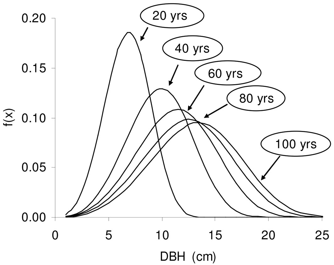
The diameter distribution models can be used independently by measuring a number of stand variables, or together with the yield table, which provides information that allows to predict the parameters of the distribution employed. The example which is provided here uses information from the yield table elaborated as part of this study for modeling the growth and production associated with the management and conservation of Tetraclinis articulata forests in Tunisia ([47]). Tab. 5 presents the predicted Weibull PDF (probability density function) parameters for different ages of the best site quality (Hd = 7 m at 50 years of age) in the case of low stand density (Reineke stand density index: SDI < 400).
Tab. 5 - Values of Weibull PDF parameters at 20, 40, 60, 80 and 100 years of age for stands with SDI < 400 and SI = 7 m (yield table).
| Stand parameters | Weibull PDF parameters | |||||
|---|---|---|---|---|---|---|
| Age | N | H m | D g | D m |
b
|
c
|
| 20 | 1909 | 3.43 | 7.21 | 6.92 | 7.51 | 3.65 |
| 40 | 1400 | 5.81 | 10.1 | 9.70 | 10.84 | 3.65 |
| 60 | 1166 | 7.74 | 12.12 | 11.61 | 12.64 | 3.58 |
| 80 | 1024 | 9.33 | 13.67 | 13.07 | 13.83 | 3.53 |
| 100 | 925 | 10.26 | 14.91 | 14.31 | 14.69 | 3.64 |
Fig. 4 shows the curves associated with these distributions and Tab. 6 represents the distribution of trees (in number and as a percentage) per diameter class for various stand ages.
Fig. 4 - Curves of diametric distribution at 20, 40, 60, 80 and 100 years by diameter (DBH, cm) for stands with SDI < 400 and SI =7 m (density of probability).
Tab. 6 - Distribution of trees at 20, 40, 60, 80 and 100 years by DBH class for stands with SDI < 400 and SI =7 m.
| DBH cm | Number of trees (Age) |
Percentage (%) (Age) |
||||||||
|---|---|---|---|---|---|---|---|---|---|---|
| 20 | 40 | 60 | 80 | 100 | 20 | 40 | 60 | 80 | 100 | |
| < 5 | 521 | 112 | 57 | 38 | 25 | 27 | 8 | 5 | 4 | 3 |
| 6-10 | 1327 | 714 | 412 | 284 | 210 | 70 | 51 | 36 | 28 | 23 |
| 11-15 | 61 | 540 | 552 | 474 | 416 | 3 | 39 | 47 | 46 | 45 |
| 16-20 | 0 | 34 | 141 | 211 | 242 | 0 | 2 | 12 | 20 | 26 |
| 21-25 | 0 | 0 | 4 | 18 | 31 | 0 | 0 | 0 | 2 | 3 |
| 26-30 | 0 | 0 | 0 | 0 | 1 | 0 | 0 | 0 | 0 | 0 |
| Total | 1909 | 1400 | 1166 | 1025 | 925 | 100 | 100 | 100 | 100 | 100 |
Based on the tree-level model attributes presented in Calama et al. ([8]), which includes height-diameter relationship, a crown attributes model and a stem curve equation, it is possible to obtain information about the distribution of end-use timber volumes, or height distribution by diameter class.
Discussion
Our Pearson’s correlations analysis results are very similar to the findings of Gorgoso et al. ([24]) for Betula alba stands in northwest Spain, using the two-parameter Weibull function, except for the parameter Ld, which expresses the logarithm of the mean diameter divided by the quadratic mean diameter. In addition, the good linear correlations which are obtained between the scale parameter (b) of the Weibull function and the stand characteristics are analogous to those observed by Campos & Leite ([9]), Leite et al. ([31]) and Binoti et al. ([4]). Linear models that relate b to the logarithm of the quadratic mean diameter (dg) show a very high determination coefficient. Similar linear models for this relationship, with values of the adjusted determination coefficient close to 99%, were obtained by Alvarez González ([1]) for Pinus pinaster in Galicia and García-Guëmes et al. ([26]) for Pinus pinea stands in Valladolid (Spain).
The results obtained in this study reveal that the Normal distribution, though less flexible, provides results which are as satisfactory as those of the Weibull distribution. Lejeune ([29]) reported similar findings for Picea abies in Belgium. However, the Weibull distribution using the maximum likelihood method to estimate parameters appears to provide a slightly superior method in terms of RMSE, MAE and EI%, especially with the parameter prediction approach.
A number of authors have reported that the two-parameter Weibull function provides the most simple and accurate approach for modelling diameter distributions, including Gorgoso ([23]), and [24]) for birch stands (Betula alba L.) in north-western Spain, Maltamo et al. ([34]) for Pinus sylvestris and Picea abies (L.) Karst. stands in Finland, Alvarez González ([1]) for Pinus pinaster stands, and Condés ([14]) for different species in Spain. Furthermore, the two-parameter Weibull function has been used in a large number of related studies due to its flexibility and high correlation of its parameters with stand characteristics ([40], [4]). Therefore, given its flexibility and the very strong correlation between the PDF parameters and stand characteristics, the two-parameter Weibull distribution, using the maximum likelihood method, appears to be the most suitable for describing diameter distributions in this study.
Gorgoso et al. ([25]) and Zhang et al. ([49]) in their studies in north west Spain and the north-eastern part of North America, respectively, obtained better results with the 3-parameter Weibull distribution, using the maximum likelihood method rather than the moments approach.
Conclusion
In this study, a model has been developed for predicting the distribution of trees by diameter class using stand variables from Tetraclinis articulata forests in north-eastern Tunisia. The developed model, used in conjunction with the previously developed models for tree level attributes ([8]), the distance-independent individual tree diameter-increment model ([46]) and the stand based growth and yield model presented in Sghaier et al. ([47]), constitutes a useful tool for the sustainable management of Tetraclinis articulata forests in north-east Tunisia.
Acknowledgements
This study (Project Number: A/017275/08) was carried out within the framework of the bilateral co-operation between Tunisia (INRGREF) and Spain (INIA), and was financed by the Ministry for Scientific Research and Technology of Tunisia (MSRT) and the Spanish Agency of International Cooperation and Development (AECID), for which they are greatly acknowledged. We also thank Adam Collins for the English review of the manuscript.
References
Gscholar
Gscholar
Gscholar
Gscholar
Gscholar
Gscholar
Gscholar
Gscholar
Gscholar
Gscholar
Gscholar
Gscholar
Online | Gscholar
CrossRef | Gscholar
Gscholar
Gscholar
Gscholar
Gscholar
CrossRef | Gscholar
CrossRef | Gscholar
Gscholar
Gscholar
CrossRef | Gscholar
Gscholar
Authors’ Info
Authors’ Affiliation
Institut National de Recherches en Génie Rural, Eaux et Forêts (INRGREF), B.P. 10, Avenue Hédi Karray 2080, Ariana (Tunisia)
Rafael Calama
Mariola Sánchez-González
INIA-CIFOR, Ctra A Coruña. km 7.5, 28040 Madrid (Spain)
Corresponding author
Paper Info
Citation
Sghaier T, Cañellas I, Calama R, Sánchez-González M (2016). Modelling diameter distribution of Tetraclinis articulata in Tunisia using normal and Weibull distributions with parameters depending on stand variables. iForest 9: 702-709. - doi: 10.3832/ifor1688-008
Academic Editor
Chris Eastaugh
Paper history
Received: Apr 25, 2015
Accepted: Dec 21, 2015
First online: May 17, 2016
Publication Date: Oct 13, 2016
Publication Time: 4.93 months
Copyright Information
© SISEF - The Italian Society of Silviculture and Forest Ecology 2016
Open Access
This article is distributed under the terms of the Creative Commons Attribution-Non Commercial 4.0 International (https://creativecommons.org/licenses/by-nc/4.0/), which permits unrestricted use, distribution, and reproduction in any medium, provided you give appropriate credit to the original author(s) and the source, provide a link to the Creative Commons license, and indicate if changes were made.

Web Metrics
Breakdown by View Type
Article Usage
Total Article Views: 52452
(from publication date up to now)
Breakdown by View Type
HTML Page Views: 42920
Abstract Page Views: 3310
PDF Downloads: 4711
Citation/Reference Downloads: 40
XML Downloads: 1471
Web Metrics
Days since publication: 3719
Overall contacts: 52452
Avg. contacts per week: 98.73
Article Citations
Article citations are based on data periodically collected from the Clarivate Web of Science web site
(last update: Mar 2025)
Total number of cites (since 2016): 10
Average cites per year: 1.00
Publication Metrics
by Dimensions ©
Articles citing this article
List of the papers citing this article based on CrossRef Cited-by.
Related Contents
iForest Similar Articles
Research Articles
Evaluation of estimation methods for fitting the three-parameter Weibull distribution to European beech forests
vol. 15, pp. 484-490 (online: 01 December 2022)
Research Articles
Developing a stand-based growth and yield model for Thuya (Tetraclinis articulata (Vahl) Mast) in Tunisia
vol. 9, pp. 79-88 (online: 23 June 2015)
Research Articles
Modeling extreme values for height distributions in Pinus pinaster, Pinus radiata and Eucalyptus globulus stands in northwestern Spain
vol. 9, pp. 23-29 (online: 25 July 2015)
Research Articles
Distribution factors of the epiphytic lichen Lobaria pulmonaria (L.) Hoffm. at local and regional spatial scales in the Caucasus: combining species distribution modelling and ecological niche theory
vol. 17, pp. 120-131 (online: 30 April 2024)
Research Articles
Local ecological niche modelling to provide suitability maps for 27 forest tree species in edge conditions
vol. 13, pp. 230-237 (online: 19 June 2020)
Research Articles
Nonlinear mixed model approaches to estimating merchantable bole volume for Pinus occidentalis
vol. 5, pp. 247-254 (online: 24 October 2012)
Research Articles
Comparison of parametric and nonparametric methods for modeling height-diameter relationships
vol. 10, pp. 1-8 (online: 19 October 2016)
Research Articles
Potential natural vegetation pattern based on major tree distribution modeling in the western Rif of Morocco
vol. 17, pp. 405-416 (online: 22 December 2024)
Research Articles
Predictive capacity of nine algorithms and an ensemble model to determine the geographic distribution of tree species
vol. 15, pp. 363-371 (online: 20 September 2022)
Research Articles
A rapid method for estimating the median diameter of the stem profile of Norway spruce (Picea abies Karst) trees
vol. 10, pp. 328-333 (online: 11 February 2017)
iForest Database Search
Search By Author
Search By Keyword
Google Scholar Search
Citing Articles
Search By Author
Search By Keywords
PubMed Search
Search By Author
Search By Keyword


