Modeling extreme values for height distributions in Pinus pinaster, Pinus radiata and Eucalyptus globulus stands in northwestern Spain
iForest - Biogeosciences and Forestry, Volume 9, Issue 1, Pages 23-29 (2015)
doi: https://doi.org/10.3832/ifor1447-008
Published: Jul 25, 2015 - Copyright © 2015 SISEF
Research Articles
Abstract
Methods of estimating extreme height values can be used in forest modeling to improve fits to the marginal distribution of heights in the following bivariate diameter-height models: the SBB Johnson’s distribution, the bivariate beta (GDB-2) distribution, the bivariate Logit-Logistic (LL-2) distribution and the power-normal (PN) distribution. Some applications to LiDAR derived data are also possible, e.g., for error calibration. Practical applications in forest management may also be considered, e.g., for pruning. In probability theory and statistics, the generalized extreme value (GEV) distribution, also known as the Fisher-Tippett distribution, is a family of continuous probability distributions that combine the Gumbel, Fréchet and Weibull distributions. This study compared the three distributions for fitting extreme values of tree heights (maximum and minimum heights), which were measured in 185 permanent research plots in Pinus pinaster Ait. stands, 97 research plots in Pinus radiata D. Don stands, and 128 research plots in Eucalyptus globulus Labill. Most of the eucalyptus stands were measured three times giving a total of 304 measurements. All plots are located in northwestern Spain. The Bias, Mean Absolute Error (MAE) and Mean Square Error (MSE) of the mean relative frequency of trees were used to evaluate the goodness-of-fit of the different functions, as well as the Kolmogorov-Smirnov statistic Dn. The Gumbel and the Weibull cumulative distribution functions (CDFs) proved suitable for describing extreme values of height distributions of the above-mentioned tree species in northwestern Spain. The Fréchet distribution was only used to model maximum values and yielded the poorest results in all cases.
Keywords
Introduction
Methods of estimating extreme values (minimum and maximum tree heights) can be applied in forest modeling, specifically for fitting bivariate height-diameter models such as the bivariate SBB Johnson’s distribution ([17]), the generalized bivariate beta distribution (GDB-2 - [19]), the bivariate Logit Logistic distribution (LL-2 - [44]) and the power-normal (PN) distribution ([24]). The accuracy of these models can be improved during fitting by choosing suitable values of the location and scale parameters, which are related to the minimum and maximum values of the marginal distribution of the SBB ([38], [18], [41], [42], [37], [49], [19]). These values also are used in LiDAR derived information, e.g., to compare the modeled values and the LiDAR-measured heights for error calibration. Knowledge of the extreme values of tree heights in forest stands is also useful for some practical applications such as pruning.
In probability theory and statistics, the generalized extreme value (GEV) distribution, also known as the Fisher-Tippett distribution, is a family of continuous probability distributions that combine the Gumbel, Fréchet and Weibull families of distributions, also known respectively as type I, II and III extreme value distributions ([31]). The Gumbel distribution ([13]) is used to model the distribution of the maximum and/or the minimum values of a number of samples of various distributions. For example, it could be used to represent the distribution of the maximum level of a river in a particular year when a list of maximum values for the past ten years were available. It is also useful for predicting the probability that an extreme earthquake, flood or other natural disaster will occur. Extreme value theory indicates that the Gumbel distribution is useful for representing the distribution of maximum values when the underlying sample data are normally or exponentially distributed. The Gumbel distribution has been variously called the log-Weibull distribution, the double exponential distribution and the Laplace distribution, and it is often incorrectly referred to as the Gompertz distribution ([47]).
Although the Fréchet distribution is named after Fréchet ([9]), who used it to model the distribution of the largest order statistic, it was further developed by Fisher & Tippett ([7]) and Gumbel ([13]). It has been shown to be useful in accelerated life testing and for modeling and analyzing rainfall, sea currents and wind speeds, as well as extreme events such as earthquakes and floods. In hydrology, the Fréchet distribution is used to model extreme events such as annual maximum one-day rainfall and river discharges ([4]). Finally, the Weibull distribution ([46]) is a simple, flexible model and it is often used in forestry studies involving diameter distributions ([1], [34], [22], [27], [48], [21], [29]). It is also used to model extreme values in many scientific disciplines.
The objective of the present study was to fit the three extreme value distributions (Gumbel, Fréchet and Weibull) to maximum and minimum tree heights in P. radiata, P. pinaster and E. globulus stands in northwestern Spain. The distributions were fitted separately as independent functions, and not jointly to yield the Generalized Extreme Value distribution.
Material and ethods
Data set
Maritime pine (P. pinaster Ait.), Monterrey pine (P. radiata D. Don) and blue gum (E. globulus Labill.) stands represent three of the most important forest resources in northwestern Spain. These species mainly occur in pure stands, although they sometimes may be found in mixed stands, and are the most commonly used species in productive stands in this area. Pure stands of maritime pine cover 217 281 ha in the region of Galicia and 22 523 ha in the adjoining region of Asturias. These stands are mainly derived from natural regeneration and occasionally from plantations. Exotic Monterrey pine plantations cover 96 177 ha in Galicia and 25 385 ha in Asturias ([23]). Pure E. globulus stands cover an area of 320 774.81 ha, 100 245.72 ha as mixed E. globulus and P. pinaster Ait. stands and 12 895.30 ha as mixed E. globulus and Q. robur L. stands in Galicia. Pure stands of E. globulus cover an area of 60 000 ha in Asturias ([23]).
The data used in this study correspond to 185 permanent research plots established in maritime pine (P. pinaster) stands, 97 plots in Monterrey pine (P. radiata) stands and 128 research plots in blue gum (E. globulus) stands. Most eucalyptus stands were measured three times, giving a total of 304 measurements. Due to the fast growth of E. globulus, the measurements are not considered repetitive and re-measurement does not affect the results. All plots are located in stands in NW Spain (in the regions of Galicia and Asturias), except for some P. radiata plots that are located in a small area of Castilla y León. In the P. pinaster stands, the plot size ranged from 375 to 900 m2, depending on the stand density, with a minimum of 30 trees per plot. In the P. radiata stands the plot size was 1000 m2, while in the E. globulus stands the plot size was about 500 m2. The minimum and the maximum heights in each distribution were extracted to form the experimental distributions of extreme values for each species. These distributions were then used for model parametrization.
The research plots used in the present study were established in stands dominated by the subject tree species (more than 85% of standing basal area) in order to cover a wide variety of combinations of age, number of trees per hectare and sites. All trees in each plot were numbered. The heights were measured with a Vertex IV hypsometer to the nearest 0.1 m. The empirical data represent non-truncated distributions.
The following stand variables were calculated from the inventory data: quadratic mean diameter, number of trees per ha, basal area and dominant height. Summary statistics of the main stand variables are shown in Tab. 1.
Tab. 1 - Descriptive statistics of main variables for the stands analyzed. (dg): quadratic mean diameter (cm); (N): trees ha-1; (H0): dominant height (m); (G:): basal area (m2 ha-1); (SD): standard deviation.
| Species | Variable | Mean | Max | Min | SD |
|---|---|---|---|---|---|
| Pinus pinaster (N=185) | dg | 20.3 | 41.5 | 10.4 | 7.1 |
| N | 1245.1 | 2480.0 | 375.0 | 483.4 | |
| H 0 | 14.1 | 30.6 | 5.4 | 4.7 | |
| G | 36.1 | 76.25 | 7.8 | 14.9 | |
| Pinus radiata (N=97) | dg | 17.8 | 25.6 | 13.4 | 3.1 |
| N | 1253.6 | 2543.3 | 596.7 | 357.0 | |
| H 0 | 18.2 | 27.0 | 13.3 | 3.1 | |
| G | 30.0 | 44.3 | 17.6 | 6.6 | |
| Eucalyptus globulus (N=304) | dg | 13.4 | 34.8 | 1.5 | 4.3 |
| N | 1174.4 | 2386.8 | 435.7 | 339.1 | |
| H 0 | 19.1 | 40.1 | 3.1 | 6.3 | |
| G | 16.5 | 63.5 | 0.15 | 8.3 |
Model fitting
The Generalized Extreme Value (GEV) distribution ([7]) has the following cumulative distribution function (CDF) for a random variable x (eqn. 1):
for 1+ ξ [(x-μ)/σ] >0, where μ is the location parameter, σ is the scale parameter and ξ is the shape parameter. The shape parameter (ξ) governs the tail behavior of the distribution. The sub-families defined by ξ = 0, ξ > 0 and ξ < 0 correspond, respectively, to the Gumbel, Fréchet and Weibull families, although the reversed Weibull is the model used to combine the three distributions in the GEV. In the present study, the distributions were fitted independently (and not jointly to yield the GEV).
The Gumbel distribution
The probably density function (PDF) and the cumulative distribution function (CDF - [13]) are formulated for a random variable as follows (eqn. 2, eqn. 3):
where z=(x-μ)/β, -∞<x<∞, μ is the mode value (location parameter), β is the scale parameter, and the standard deviation (σ) is (eqn. 4):
The function was fitted using a location parameter (μÂ) recovered from the experimental mean (d) and standard deviation (σ) of the distributions, with the following expression (eqn. 5):
where γ is the Euler-Mascheroni constant (eqn. 6):
The Fréchet distribution
The Fréchet distribution is a special case of the generalized extreme value distribution. This type-II extreme value distribution is equivalent to the inverse values of a standard Weibull distribution. The probability density function (PDF) and the cumulative distribution function (CDF) for the Fréchet distribution ([9]) used for the largest order statistic are as follows (eqn. 7, eqn. 8):
where α > 0 is the shape parameter. In this case, the distribution is generalized to include a location parameter m (the minimum value of the distribution) and a scale parameter s > 0.
Parameters of the Fréchet distribution were obtained using the method of moments: mean dÌÂ and variance σ2, with the following equations (eqn. 9):
for α>1 and (eqn. 10):
for α>2. eqn. 9 and 10 were solved using iterative procedures with the solver function of Microsoft Excel®.
The Weibull distribution
The CDF for the three-parameter Weibull CDF is obtained by integrating the Weibull PDF. For a continuous random variable x it has the following expression (eqn. 11, eqn. 12):
where μ is the location parameter, β is the scale parameter and α is the shape parameter. The scale parameter β and the shape parameter α of the Weibull distribution were obtained by the method of moments. The location parameter μ was predetermined as the minimum value in each distribution, and 1 m height classes were used in the distributions.
In this study, the method of moments was chosen for fitting because the moments of the distribution were also used for fitting the Gumbel and Fréchet CDFs. Such method has been previously applied ([26], [6], [40], [11]), and is based on the relationship between the parameters of the Weibull function and the first and second moments of the diameter distribution (mean diameter and variance, respectively - eqn. 13, eqn. 14):
where d is the arithmetic mean diameter of the distribution, σ2 is the variance and Γ is the Gamma function. eqn. 14 was resolved by a bisection iterative procedure ([10]).
All distributions were fitted using the software SAS/STATTM ([36]).
Goodness-of-fit evaluation
The consistency of the model and the fitting method were evaluated using the Kolmogorov-Smirnov statistic (Dn). For a given cumulative distribution function F(x): Dn = supx|Fn(x) - F0(x)|, where supx is the supreme of the set of distances. This value was calculated as follows (eqn. 15):
where the cumulative observed frequency Fn(xi) is compared with the cumulative estimated frequency F0(xj).
Bias, mean absolute error (MAE) and mean square error (MSE) were also used as goodness-of-fit measures and were expressed as follows (eqn. 16, eqn. 17, eqn. 18):
where Yi is the relative frequency of trees observed value in each height class, Yi is the theoretical value predicted by the model, and N is the number of data points.
The bias, MAE and MSE values were calculated for each fit as mean relative frequency of trees.
Results
The main descriptive statistics of the distributions under study, including the mean, maximum and minimum values, 25th, 50th and 75th percentiles, standard deviation, and skewness and kurtosis coefficients, are summarized in Tab. 2. The parameter estimates of the Fréchet, Gumbel and Weibull distributions are shown in Tab. 3. The mean values of bias, mean absolute error (MAE) and mean square error (MSE) in relative frequency of trees and the Kolmogorov-Smirnov statistic (Dn) for the fits with the distributions in forest stands of the three species in NW Spain are shown in Tab. 4.
Tab. 2 - Main descriptive statistics of the distributions studied: mean, maximum and minimum values, 25th, 50th and 75th percentiles, standard deviation and skewness and kurtosis coefficients. (hmax); maximum height; (hmin): minimum height; (P25): 25th percentile; (P50): 50th percentile; (P75): 75th percentile; (Sk): skewness coefficient; (Kur): kurtosis coefficient.
| Species | Variable | Mean | Max | Min | P25 | P50 | P75 | SD | Sk | Kur |
|---|---|---|---|---|---|---|---|---|---|---|
| Pinus pinaster | h max |
16.32 | 36.0 | 6.1 | 12.2 | 15.5 | 18.9 | 5.59 | 0.95 | 0.81 |
h min |
7.41 | 16.7 | 1.4 | 4.9 | 6.6 | 9.5 | 3.23 | 0.72 | -0.14 | |
| Pinus radiata | h max |
21.13 | 31.7 | 15.2 | 18.4 | 20.7 | 23.2 | 3.45 | 0.72 | 0.56 |
h min |
6.40 | 13.6 | 2.6 | 4.5 | 6.2 | 7.5 | 2.22 | 0.81 | 0.69 | |
| Eucalyptus globulus | h max |
20.98 | 42.6 | 3.3 | 16.3 | 20.9 | 25.2 | 6.91 | 0.32 | 0.49 |
h min |
5.23 | 14.3 | 0.6 | 3.5 | 4.8 | 6.9 | 2.48 | 0.65 | 0.41 |
Tab. 3 - Parameter values for the Gumbel, Fréchet and Weibull distributions fitted using the moments approach. (hmax); maximum height; (hmin): minimum height; (a): values of the parameter m; (b): values of the parameter s.
| Distribution | Species | Variable |
μ
|
β
|
α
|
|---|---|---|---|---|---|
| Gumbel | Pinus pinaster | h max |
13.81 | 4.36 | - |
h min |
5.96 | 2.52 | - | ||
| Pinus radiata | h max |
19.57 | 2.69 | - | |
h min |
5.40 | 1.73 | - | ||
| Eucalyptus globulus | h max |
17.88 | 5.39 | - | |
h min |
4.12 | 1.93 | - | ||
| Fréchet | Pinus pinaster | h max |
6.1 a | 7.93 b | 3.39 |
| Pinus radiata | h max |
15.2 a | 4.62 b | 3.30 | |
| Eucalyptus globulus | h max |
3.3 a | 14.66 b | 4.24 | |
| Weibull | Pinus pinaster | h max |
6.1 | 11.52 | 1.90 |
h min |
1.4 | 6.78 | 1.94 | ||
| Pinus radiata | h max |
15.2 | 6.66 | 1.77 | |
h min |
2.6 | 4.27 | 1.76 | ||
| Eucalyptus globulus | h max |
3.3 | 19.87 | 2.77 | |
h min |
0.6 | 5.23 | 1.95 |
Tab. 4 - Mean values of bias, mean absolute error (MAE), mean square error (MSE) and Kolmogorov-Smirnov statistic (Dn). (hmax); maximum height; (hmin): minimum height.
| Species | Variable | Distribution | Bias | MAE | MSE | D n |
|---|---|---|---|---|---|---|
| Pinus pinaster | h max |
Gumbel | 0.01353 | 0.01662 | 0.00053 | 0.06139 |
| Fréchet | 0.01006 | 0.04593 | 0.00478 | 0.20288 | ||
| Weibull | 0.01406 | 0.01863 | 0.00076 | 0.07219 | ||
h min |
Gumbel | 0.02630 | 0.02931 | 0.00182 | 0.09556 | |
| Weibull | 0.02767 | 0.02873 | 0.00176 | 0.09507 | ||
| Pinus radiata | h max |
Gumbel | 0.02745 | 0.02896 | 0.00181 | 0.11332 |
| Fréchet | 0.02871 | 0.06182 | 0.00991 | 0.27513 | ||
| Weibull | 0.02838 | 0.02935 | 0.00147 | 0.09595 | ||
h min |
Gumbel | 0.03655 | 0.03655 | 0.00211 | 0.12012 | |
| Weibull | 0.03718 | 0.03718 | 0.00209 | 0.11979 | ||
| Eucalyptus globulus | h max |
Gumbel | 0.01033 | 0.02316 | 0.00089 | 0.12639 |
| Fréchet | 0.00713 | 0.04421 | 0.00414 | 0.18785 | ||
| Weibull | 0.01154 | 0.01666 | 0.00050 | 0.07409 | ||
h min |
Gumbel | 0.02965 | 0.02965 | 0.00161 | 0.12046 | |
| Weibull | 0.03003 | 0.03007 | 0.00165 | 0.11230 |
The mean value of the mean square error (MSE) in the relative frequency of number of trees in each diameter class for the fits with the three distributions is shown in Fig. 1. The observed and predicted distributions of maximum and minimum heights for maritime pine, Monterrey pine and blue gum are shown in Fig. 2.
Fig. 1 - Mean values of MSE in each height class in the fits with the Gumbel, Weibull and Fréchet CDFs used for describing extreme values of heights in three tree species from NW Spain. (a-b): Pinus pinaster; (c-d): Pinus radiata; (e-f): Eucalyptus globulus; (a-c-e): maximum heights (m); (b-d-f): minimum heights (m).
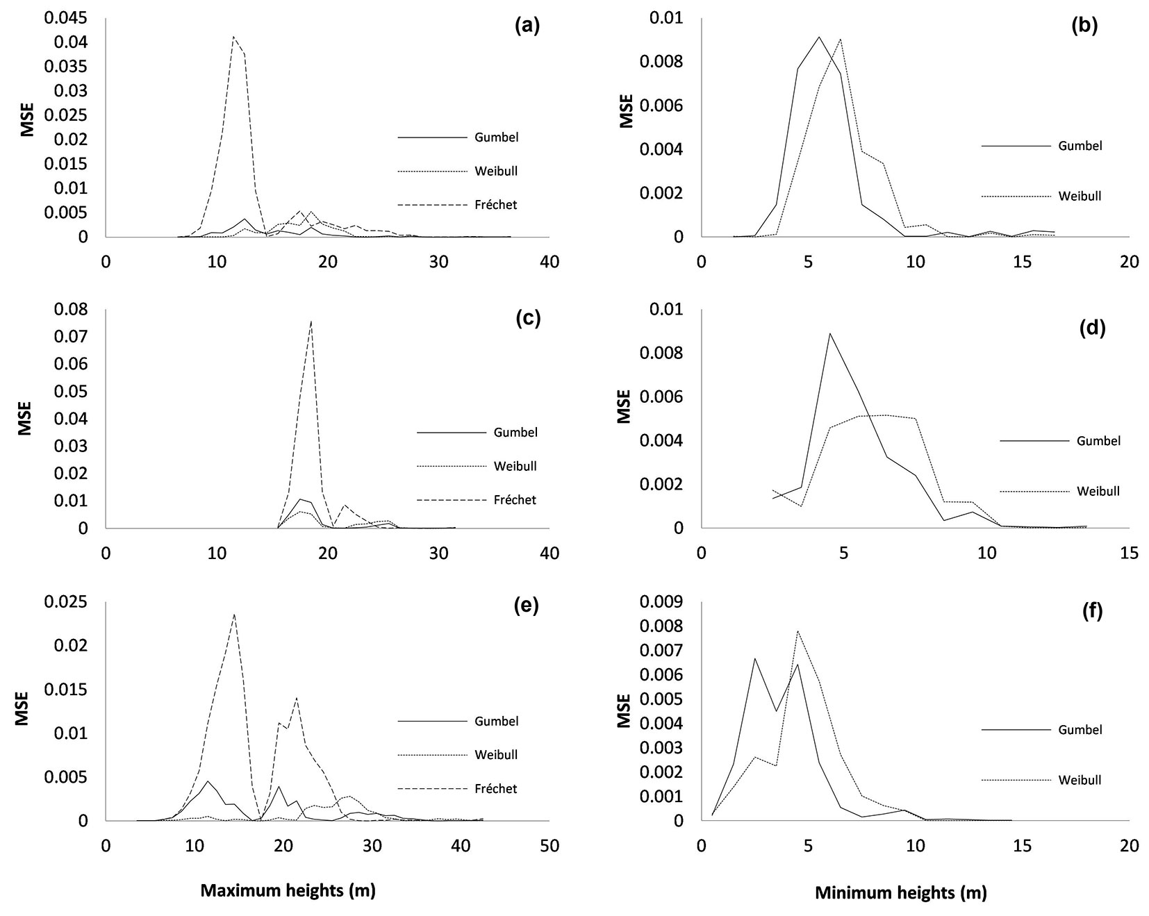
Fig. 2 - Observed and fitted cumulative distributions, for which the Gumbel, Weibull and Fréchet CDFs were used to describe extreme values of heights in three tree species from NW Spain. (a-b): Pinus pinaster; (c-d): Pinus radiata; (e-f): Eucalyptus globulus; (a-c-e): maximum heights (m); (b-d-f): minimum heights (m).
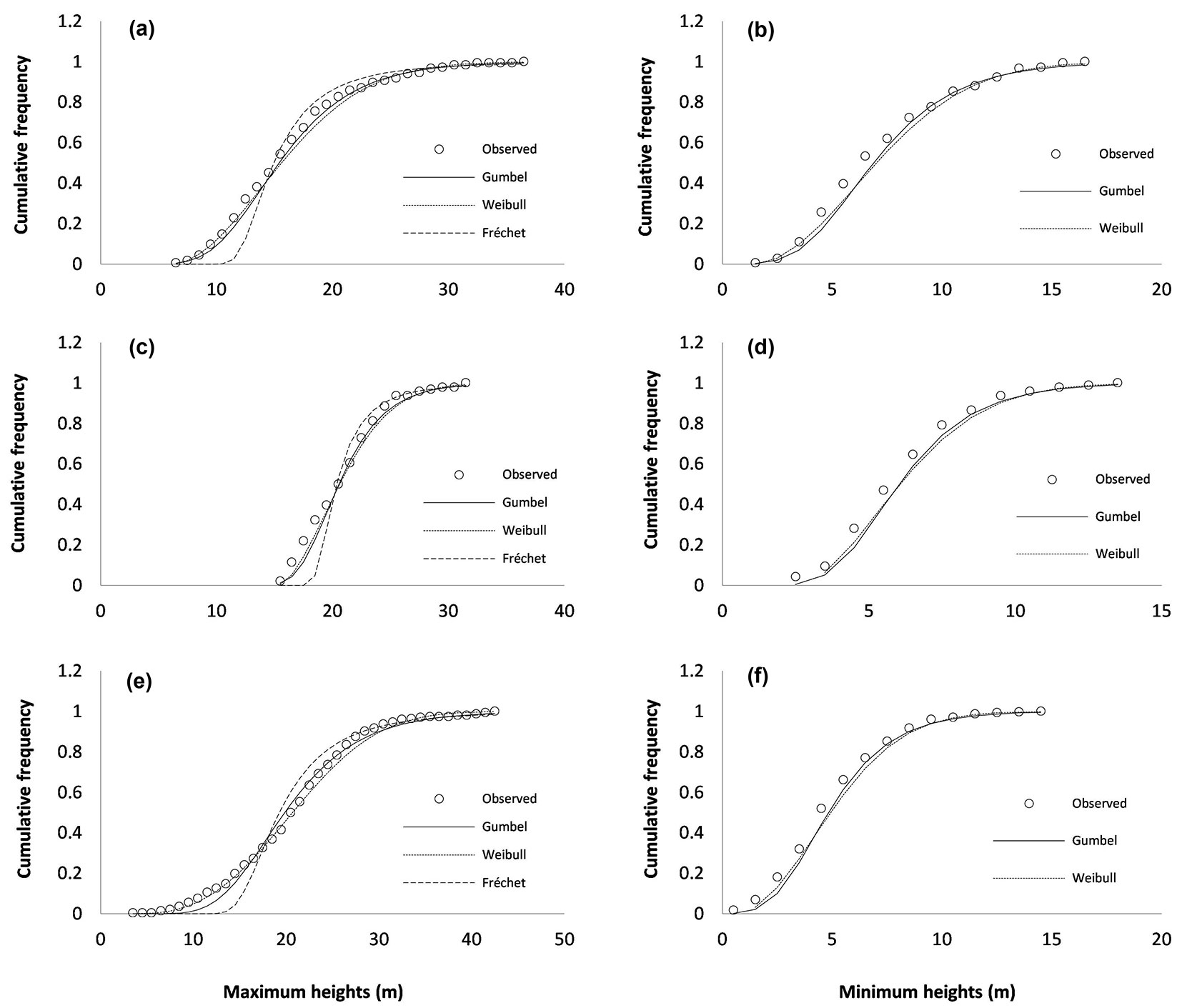
Results showed that the Gumbel and the Weibull CDFs are suitable for describing extreme tree heights in P. pinaster, P. radiata and E. globulus stands in northwestern Spain (Tab. 4, Fig. 1, Fig. 2). The Fréchet distribution used for the maximum values yielded the poorest results in all cases under study. It tended to underestimate frequencies in the lower half of the data range and then to overestimate the frequencies in the upper half.
The Gumbel and the Weibull distributions generally yielded similar results for the fits to distributions of minimum heights, as indicated by the main statistics used to compare the results (Kolomogorov-Smirnov Dn statistic and mean square error, MSE). The bias may be less useful because errors with different signs tend to cancel out, thus confounding the overall value. The results were slighter better for maximum than for minimum heights. The Gumbel CDF was the most suitable model for P. pinaster stands, while the Weibull CDF was the most appropriate for P. radiata and E. globulus stands.
Discussion
In this study, extreme (maximum and minimum) tree height data from permanent plots of P. pinaster, P. radiata and E. globulus species - representing the heterogeneity and complexity of forest stands in the study area - were fitted using three extreme value distributions. This is a novel approach in forest modeling.
Knowledge of the distributions of the maximum and minimum tree heights in forest stands is useful in forest modeling, for example, for improving fits of the bivariate distribution functions. In the Johnson’s SBB distribution, the location parameter (εh) of the Johnson’s SB marginal distribution of heights is usually fixed as the minimum height of the distribution, while the scale parameter (λh) of the same marginal distribution of heights is considered as the range of the distributions, i.e., as maximum height - minimum height ([38], [42], [19], [49]). Some authors have considered a value of 1.3 for the location parameter when fitting the marginal distribution of heights ([39], [2]). However, Mønness ([24]) compared the Johnson’s SB and the power-normal (PN) distributions fitted to diameters and heights of trees in forest stands by fixing the location parameter of the Johnson’s SB distribution of heights as Hmin - (Hmax - Hmin)/n.
The final accuracy of the bivariate SBB distribution could be improved by increasing the accuracy of the fits of the Johnson’s SB marginal distributions of diameters and heights. As for diameters, several studies have fixed different location parameters of the Johnson’s SB in relation to the minimum diameter of the distribution ([18], [48], [30], [8], [11]). However, similar studies have not been applied to the SBB model, which could be improved by a similar approach applied to the marginal distribution of heights. In this case, knowledge of the distribution of minimum heights may be useful for choosing the most suitable location parameter (εh) instead of trying to use complicated algorithms to predetermine it. The value of the scale parameter of the extreme value distributions fitted in the present study could help in choosing the ideal location parameter in these marginal distributions by fixing it as a fraction of the minimum diameter observed: this fraction is small when the scale parameter of the extreme value distribution is low ([12]).
Similar applications of extreme height distributions could also be used with the generalized beta distribution (GDB-2) and the marginal distribution of both diameters and heights, as reported by Li et al. ([19]). These authors estimated two of the four parameters of each marginal GDB-2 (β1, β2, β3 and β4) by substituting βÌÂ1 = xmin and βÌÂ2 = xmax - βÌÂ1, where xmin and xmax are the minimum and the maximum values of the marginal distributions of heights and diameters. Wang & Rennolls ([44]) presented a bivariate distribution (LL-2) based on the univariate Logit-Logistic ([43]), which is obtained by the parametrization of the Johnson’s SB distribution. The location parameter is the same in both distributions.
Airborne light detection and ranging (LiDAR) also uses maximum and minimum heights and has proven useful for characterizing the forest canopy in three dimensions ([45]). Since the first application of airborne LiDAR in forestry over a decade ago ([28]), the technology has been widely used to quantify the spatial variation in tree height and crown dimensions at resolutions ranging from stand level ([14], [25]), to plot level ([16], [20], [33]) and individual tree level ([3], [5], [15], [32], [35]). Comparison of the maximum heights estimated from the extreme value distributions with the maximum heights measured by LiDAR at individual tree level is useful, mainly for error calibration, which enables recalculation of all heights measured by LiDAR and estimation of the stand structure.
The following procedure is commonly used to correct errors in LiDAR derived data. The LiDAR data are obtained for the study area and the tree heights are measured in the field (usually with a Vertex hypsometer). The LiDAR technique is used to construct a Digital Terrain Model (DTM) and a Digital Surface Model (DSM) and to determine the tree heights from the vertical difference between such models (DSM-DTM). The LiDAR-derived heights are usually smaller than the field-measured heights. A regression model is then fitted to both sets of height data to correct the LiDAR-measured heights. The accuracy of this model is assessed using the coefficient of determination.
Several other applications of our results may be also identified, such as pruning. The most appropriate timing of pruning is a very important decision that depends on the height and/or diameter of the tree. In general, the height criterion is easier and cheaper to establish in the field. Pruning is carried out in P. pinaster and P. radiata stands in NW Spain to improve the quality of the wood mainly for the saw and veneer industries. To prevent growth reduction, less than 33% of the total height of the tree should be removed in young stands and less than 50% in old stands. Thus, the first pruning may be applied to trees of minimum height 8 m, with 2.5-2.7 m of the tree removed.
Conclusion
In conclusion, the three extreme value distributions (Gumbel, Fréchet and Weibull) were fitted independently to observed maximum and minimum heights in P. pinaster, P. radiata and E. globulus stands in northwestern Spain, in a novel approach in the field of forest modeling. The most common potential applications are in forest modeling, for fitting bivariate height-diameter distributions, and in other fields where extreme values are used, such as LiDAR. Practical applications in forest management may also be considered, for example, for pruning.
Acknowledgements
The authors thank forestry students from the Universities of Oviedo and Santiago de Compostela who participated in the fieldwork.
The study was financially supported by the Gobierno del Principado de Asturias through the project entitled “Estudio del crecimiento y producción de Pinus pinaster Ait. en Asturias” (CN-07-094); by the Ministerio de Ciencia e Innovación through the project entitled “Influencia de los tratamientos selvícolas de claras en la producción, estabilidad mecánica y riesgo de incendios forestales en masas de Pinus radiata D. Don y Pinus pinaster Ait. en el Noroeste de España” (AGL2008-02259), and an ongoing research project entitled “Growth and yield modelling of clonal and seedling plantations of Eucalyptus globulus Labill. of NW Spain” (code AGL2010-22308-C02-01), funded by the Ministry of Science and Innovation of Spain and the European Union through the ERDF programme for the period 2011-2013.
The Sustainable Forest Management Unit (UXFS) is funded by the Xunta de Galicia (“Consolidation and Structuring Program of Competitive Research Units 2011”) and by the ERDF.
References
Online | Gscholar
Gscholar
Gscholar
Gscholar
Gscholar
Gscholar
Gscholar
Gscholar
Authors’ Info
Authors’ Affiliation
Departamento de Biología de Organismos y Sistemas, Universidad de Oviedo, Escuela Politécnica de Mieres, c/ Gonzalo Gutiérrez Quirós s/n, E-33600 Mieres, Asturias (Spain)
Alberto Rojo-Alboreca
Unidade de Xestión Forestal Sostible (UXFS), Departamento de Enxeñaría Agroforestal, Universidade de Santiago de Compostela, Escola Politécnica Superior, Campus Universitario s/n, E-27002 Lugo, Galicia (Spain)
Corresponding author
Paper Info
Citation
Gorgoso-Varela JJ, García-Villabrille JD, Rojo-Alboreca A (2015). Modeling extreme values for height distributions in Pinus pinaster, Pinus radiata and Eucalyptus globulus stands in northwestern Spain. iForest 9: 23-29. - doi: 10.3832/ifor1447-008
Academic Editor
Emanuele Lingua
Paper history
Received: Sep 18, 2014
Accepted: Mar 21, 2015
First online: Jul 25, 2015
Publication Date: Feb 21, 2016
Publication Time: 4.20 months
Copyright Information
© SISEF - The Italian Society of Silviculture and Forest Ecology 2015
Open Access
This article is distributed under the terms of the Creative Commons Attribution-Non Commercial 4.0 International (https://creativecommons.org/licenses/by-nc/4.0/), which permits unrestricted use, distribution, and reproduction in any medium, provided you give appropriate credit to the original author(s) and the source, provide a link to the Creative Commons license, and indicate if changes were made.

Web Metrics
Breakdown by View Type
Article Usage
Total Article Views: 54254
(from publication date up to now)
Breakdown by View Type
HTML Page Views: 45029
Abstract Page Views: 3274
PDF Downloads: 4434
Citation/Reference Downloads: 23
XML Downloads: 1494
Web Metrics
Days since publication: 3980
Overall contacts: 54254
Avg. contacts per week: 95.42
Article Citations
Article citations are based on data periodically collected from the Clarivate Web of Science web site
(last update: Mar 2025)
Total number of cites (since 2016): 6
Average cites per year: 0.60
Publication Metrics
by Dimensions ©
Articles citing this article
List of the papers citing this article based on CrossRef Cited-by.
Related Contents
iForest Similar Articles
Research Articles
Modelling diameter distribution of Tetraclinis articulata in Tunisia using normal and Weibull distributions with parameters depending on stand variables
vol. 9, pp. 702-709 (online: 17 May 2016)
Research Articles
Evaluation of estimation methods for fitting the three-parameter Weibull distribution to European beech forests
vol. 15, pp. 484-490 (online: 01 December 2022)
Short Communications
When a definition makes the difference: operative issues about tree height measures from RPAS-derived CHMs
vol. 13, pp. 404-408 (online: 03 September 2020)
Research Articles
Climatic factors defining the height growth curve of forest species
vol. 10, pp. 547-553 (online: 05 May 2017)
Technical Advances
Forest stand height determination from low point density airborne laser scanning data in Roznava Forest enterprise zone (Slovakia)
vol. 6, pp. 48-54 (online: 21 January 2013)
Research Articles
Local ecological niche modelling to provide suitability maps for 27 forest tree species in edge conditions
vol. 13, pp. 230-237 (online: 19 June 2020)
Research Articles
Genetic control of intra-annual height growth in 6-year-old Norway spruce progenies in Latvia
vol. 12, pp. 214-219 (online: 25 April 2019)
Research Articles
Total tree height predictions via parametric and artificial neural network modeling approaches
vol. 15, pp. 95-105 (online: 21 March 2022)
Research Articles
Temperatures at the margins of a young spruce stand in relation to aboveground height
vol. 6, pp. 302-309 (online: 16 July 2013)
Research Articles
Three-dimensional forest stand height map production utilizing airborne laser scanning dense point clouds and precise quality evaluation
vol. 10, pp. 491-497 (online: 12 April 2017)
iForest Database Search
Search By Author
Search By Keyword
Google Scholar Search
Citing Articles
Search By Author
Search By Keywords
PubMed Search
Search By Author
Search By Keyword


