Properties and prediction accuracy of a sigmoid function of time-determinate growth
iForest - Biogeosciences and Forestry, Volume 8, Issue 5, Pages 631-637 (2015)
doi: https://doi.org/10.3832/ifor1243-007
Published: Jan 13, 2015 - Copyright © 2015 SISEF
Research Articles
Abstract
The properties and short-term prediction accuracy of mathematical model of sigmoid time-determinate growth, denoted as “KM-function”, are presented. Comparative mathematical analysis of the function revealed that it is a model of asymmetrical sigmoid growth, which starts at zero size of an organism and terminates when it reaches its final size. The function assumes a finite length of the growth period and includes a parameter interpretable as the expected lifespan of the organism. Moreover, the possibility for growth curve inflexion at any age is possible, so the function can be used for modelling of S-shaped growth trajectories with various degree of asymmetry. These good theoretical predispositions for realistic growth predictions were empirically evaluated. The KM-function used in three and four-parameter forms was compared with three classical (Richards, Korf and Weibull) growth functions employing two parameterisation methods - nonlinear least squares (NLS) and Bayesian method. The evaluation was conducted on the basis of the tree diameter series obtained from stem analyses. The main empirical findings are: (i) if the minimisation of the prediction bias is required, the KM-function in three-parameter form in connection with Bayes parameterisation can be recommended; (ii) if the minimisation of root square error (RMSE) is required, the best short-term prediction results for a particular dataset were obtained with four-parameter Weibull function employing NLS parameterisation; (iii) moreover, three-parameter functions parameterised by Bayesian methods show a considerably smaller RMSE by 15-25% as well as smaller biases by 40-60% than four-parameter functions employing NLS. Overall, all analyses confirmed relative usefulness of the KM-function in comparison with classical growth functions, especially in connection with Bayesian parameterisation.
Keywords
Growth Function, Determinate Growth, Nonlinear Least Squares, Bayes, Prediction
Introduction
Changes in plant size over the lifespan are typically characterized by an S-shaped growth trajectory ([21], [35], [38]). Growth functions represent simple, non-linear equations describing the sigmoidal change in size of an individual or population with time. Their mathematical forms are derived empirically or conceived from the biological knowledge of the growth of living organisms ([2]). Historically, the Gompertz, logistic, Mitscherlich or Korf’s growth models rank among the most successful functions used in modeling the plant growth ([10], [15], [19], [33]). Currently, the most used growth model is the Richards’ function ([23]) which was obtained by the generalization of the Bertallanffy’s growth function ([1]). Among the growth functions with unique properties, the Weibull’s or Sloboda’s equations and the increasingly popular Schnute’s growth function are also worth to be mentioned ([34], [29], [28]). A comprehensive survey of the historical background, the mathematical and statistical properties of the mentioned growth functions may be found in the works by Zeide ([38]), Seber & Wild ([24]), Tsoularis & Wallace ([31]) and Karkach ([13]).
The application of growth functions is now more common than ever. Growth functions are based on relatively simple equations with a limited number of parameters; nonetheless, they show a good ability to encompass complicated growth processes ([40]). A direct prediction of the integral quantities of growth at individual or population level by means of simpler growth functions can be more precise than prediction from the sum of the individual components of growth (cells, tissues and organs) obtained by more complicated process models. In general, this can be considered a major paradox of ecological modeling and represents a considerable challenge to plant ecology science ([21], [24], [39]).
From a mathematical point of view, each growth function suitable for the description of sigmoid growth must be able to describe a nonlinear, monotonically increasing growth pattern having a concave shape along the early life stages. At later stages, this turns into a convex function which approaches a final asymptote. For these reasons, growth functions are characterized by the inclusion of three or four parameters defining the position and shape of the growth curve ([8], [9]). In general, the asymptotic parameter β0 is present in all classical growth functions ([3]), and represents the limit (eqn. 1):
Hence, β0 is the asymptotic value which the growth function approaches towards the end of an organism’s life, and which the growth function will reach after an infinite growth period.
A detailed analysis on the mathematical structure of some important growth functions by Shvets & Zeide ([27]) reported that even after 200 years of intensive research, there is still opportunity for improvement of the mathematical structure of existing growth functions. Karkach ([13]) distinguishes two general growth types: determinate and non-determinate growth. The former applies when the growth of an organism terminates at a certain development stage or at a final (maximum) size, whereas non-determinate growth continues throughout the organism’s lifespan, regardless of the degree of physiological maturity attained. Due to the existence of the asymptotic parameter β0, all classical growth functions are non-determinate growth models that implicitly entail an infinite length of the growth period. This fact is clearly not consistent with the biological reality. The use of an asymptotic growth function for a finite life length of every living organism is possible only because they predict very small, practically negligible growth rates at the oldest ages.
Recently, two attempts to solve the aforementioned issue has been reported in the literature. Yin et al. ([36]) proposed a new flexibile empirical function of sigmoid determinate growth, obtained by modifying the probability density function of the beta distribution. Sedmák & Scheer ([26]) derived another sigmoid function of determinate growth, called KM-function, based on a modification of the Kumaraswamy’s distribution function ([16]). Generally, both probability distributions are suitable for double-bounded random variables, and consequently they are theoretically well-suited for the description of determinate growth within a finite period of time.
Growth functions are used as semi-empirical models whose parameters are inferred from empirical measurements of the growth of an organism ([13], [27], [40]). Their parameter estimations are carried out by means of different theoretical methods, mainly based on non-linear regressions. A wide range of methods of classic (Fisherian) frequentist statistics ([24]) or the alternative Bayesian statistics ([5]) are currently used to this purpose.
To estimate the parameters in the regression models, the most common methods used by the frequentist school are the maximum likelihood estimation (MLE) and the ordinary least squares (OLS). The OLS method is derived from the MLE by introducing the simplified assumptions of normality, variance homogeneity and uncorrelatedness of residual deviations of the regression model. Using the OLS method, parameter estimation is almost exclusively related to the solution of a set of non-linear equations by numerical techniques. In such cases, the OLS method is also called nonlinear least squares (NLS) estimation.
An alternative method for the estimation of growth function parameters is based on a Bayesian approach. The basic difference between Fisherian and Bayesian statistical schools relies on a different understanding of the probability concept ([6]). In the Bayesian estimation, the a priori joint probability distribution of possible parameter values in the model is combined with information from data represented by the likelihood function.
The objective of this study was to assess the performances of the KM-function in modeling the sigmoid determinate growth in living organisms and to analyse its theoretical properties. The analysis was carried out by comparing the properties and prediction accuracy of the KM-function with those of selected classical growth functions. The statistical properties of growth functions were compared based on empirical data, made by diameter growth series of individual trees obtained from stem analyses. Two methods of statistical parametrization were used: the classic nonlinear least squares method, and the Bayesian parametrization method based on the Markov chain Monte Carlo procedure.
Material and methods
Growth functions included into comparison
Tab. 1 - List of the growth models compared in this study.
| Model (abbr) | Integral form | Source |
|---|---|---|
| KM-function (KM3) | y = ymax [1-(1-(t/500)b)c] |
Kumaraswamy ([16]) |
| KM-function (KM4) | y = ymax[1-(1-(t/tmax)b)c] |
Kumaraswamy ([16]) |
| Richards function (R3) | y = ymax(1-e-bt)c |
Zeide ([38]) |
| Richards function (R4) | y = ymax (1-de-bt)c |
Richards ([23]), Fitzhugh ([9]) |
| Korf function (KF3) | y = ymax e(-bt)^c |
Korf ([15]), Li et al. ([17]) |
| Weibull function (W4) | y = a - de-(bt)^c |
Weibull ([34]), Ratkowsky ([22]) |
An overview of the growth functions used in this study is reported in Tab. 1. The first function was a time-determinate KM-function with the following integral form (eqn. 2):
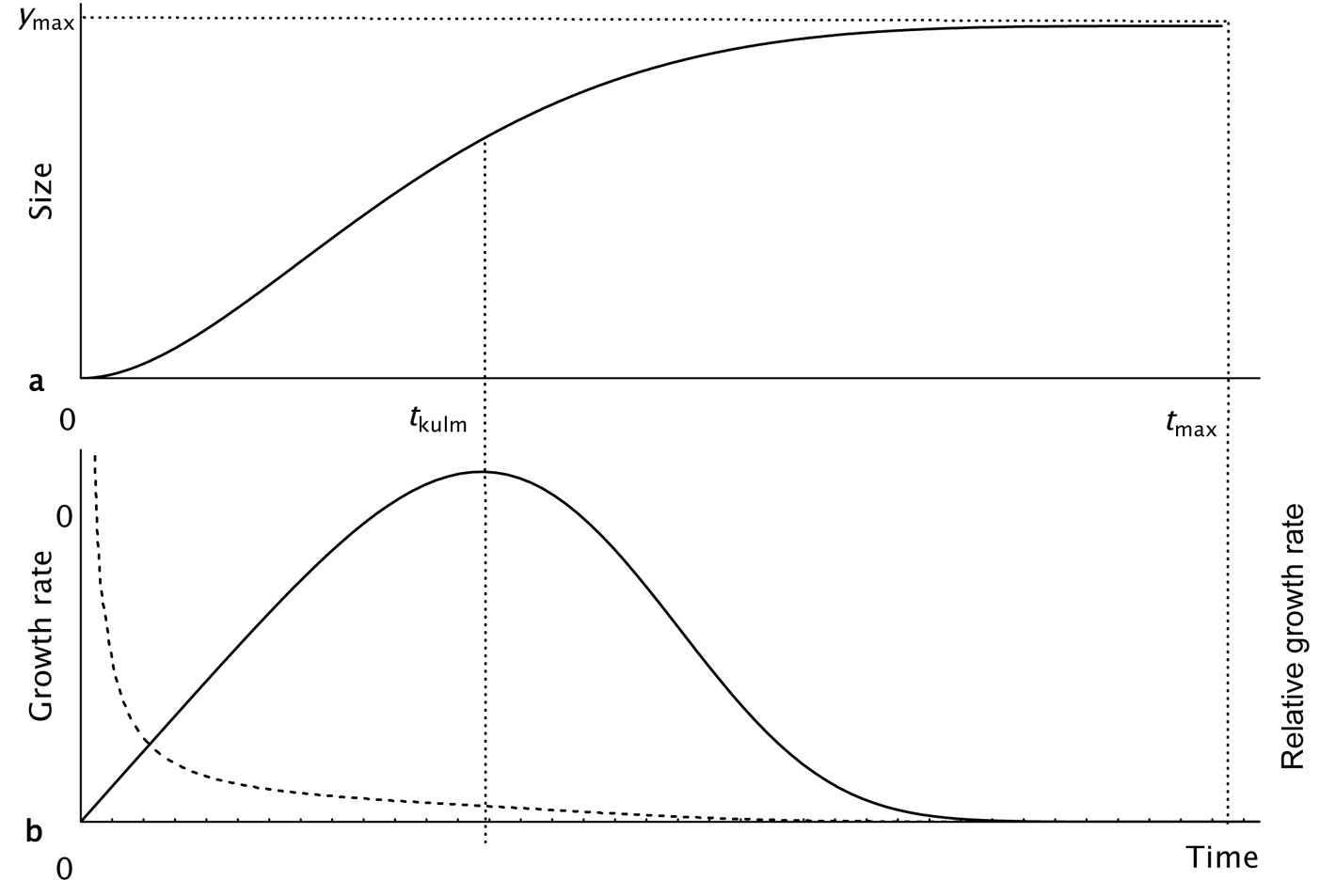
where 0 ≤ t ≤ tmax, tmax > 0, ymax > 0, b > 0, c > 0. The parameter ymax is interpreted as the final (maximum) size of an organism attained at the age tmax. If the parameter tmax is fixed on the basis of a clear biological interpretation, the new function will have only three parameters. The parameters b and c determine the position of its inflexion point within the life cycle. The growth rate equation can be obtained by derivation from eqn. 2 as follows (eqn. 3):
A typical course of the KM-function over time and that of the derived absolute and relative growth rates (RGR) are shown in Fig. 1a and Fig. 1b. In this study, the KM-function was used in two parametrization forms with a different number of parameters (Tab. 1). The three-parameter form was derived from the four-parameter version by fixing the parameter tmax to a value of 500 years on the basis of the maximum lifetime estimated for beech trees in Slovakia ([20]).
Fig. 1 - Growth trajectory described by the sigmoid KM-function. (a): Growth period starts at t=0 and ends at the age tmax, at which the exact final value is reached; (b): full and broken lines show the corresponding courses of growth and relative growth rates, which are exactly equal to zero at the age tmax.
The Richards’ function is one of the most important growth models of the exponential decline type sensu Zeide ([38]), and represents one of the most used growth models worldwide. Its popularity stems from the excellent flexibility, along with a relatively good extrapolation capability. Similarly to the KM-function, the Richards’ function is also used in its forms including three or four parameters.
The Korf’s growth function belongs to the power decline type sensu Zeide ([38]), and it is considered as the most suited to forestry conditions of Slovakia. It was used for the construction of the national growth and yield tables ([11]). According to Zeide ([37]), this function is especially suitable for the description of the diameter of a fixed number of trees, as it is more accurate than other traditional growth functions.
The Weibull’s growth function does not belong to any of the aforementioned classification sensu Zeide (1989). From a practical point of view, this function has the same advantages as the Richards’ function, and it was included in the list of Tab. 1 because it was derived exclusively in an empirical way, just as the KM-function.
All the classical growth functions described above share the common feature of being time-non-determinate growth models with an asymptotic behavior.
Dataset
The empirical dataset used in this study consisted of stem analyses for 67 beech trees cut in an 80-160 years-old mature forest stand growing in a good-quality site. The analysis of the selected growth functions and parametrization methods was performed on growth series at time intervals of five years based on the diameter at breast height (d1.3) measured to the nearest 1 mm. Current and mean annual increments were inferred from diameter growth data. Growth and increment curves were subjected to graphical analysis, revealing two episodes of abrupt increases in current increment along the stand history. The first episode was interpreted as due to an intensive thinning carried out prior to the culmination of current increments at the age of 50-70 years, while the other was at the beginning of the natural regeneration step at the age of 120-140 years. From a modeling point of view, the increase of tree growth at later stages due to seeding felling is in contradiction with the sigmoid-shaped growth models, that predict a reduction of current increment at older ages. Therefore, each diameter growth series was truncated, considering only the data prior to the start of the stand’s natural regeneration (identified at age 120 years). Moreover, data from trees with age < 20 years were excluded from growth series, since their diameters were affected by rather high measurement errors. In total, 67 growth series with age ranging from 20 to 115 years were included in the analysis. Since data were grouped in 5 years intervals, each individual growth series was composed by 19 measured diameters. More detailed information on individual series and discrete events along the stand history are given in Tab. 2.
Tab. 2 - Main statistics of the empirical growth series analyzed. (SD): Standard deviation; (dbh): diameter at the breast height.
| Statistics | Current increment culmination (yrs) | Mean increment culmination (yrs) | Age of 1st release (yrs) |
Beginning of regeneration (yrs) |
Cut down age (yrs) | Cut down dbh (cm) |
|---|---|---|---|---|---|---|
| Minimum | 27 | 33 | 25 | 75 | 85 | 17.3 |
| Mean ± SD | 72 ± 14 | 95 ± 20 | 61 ± 18 | 114 ± 18 | 131 ± 17 | 37.1 ± 9.7 |
| Maximum | 100 | 145 | 110 | 150 | 165 | 54.4 |
Error analysis
Performances of growth functions were assessed by estimating the bias and accuracy of short-term (5 years) predictions of tree diameter growth. Comparison of observed vs. predicted values for the variables considered represent a commonly-used, simple method to evaluate growth models ([21], [32]). Model validation through the analysis of deviations of projected values from empirical data, allows an objective estimation of the ability of growth functions to capture meaningful biological trends, and extrapolate growth changes over time, thus assessing its suitability to modeling purposes ([7], [41]).
Each growth series was divided into two parts for parametrization and validation purposes. The parametrization step was carried out on sequences of 18 measurements at the age ranging from 25 to 110 years covering all the life stages (juvenility, maturity, senescence). The validation step was carried out on one measurement at the age of 115 years. This measurement was omitted from the existing growth series and used for comparison of real diameter at this age with the diameter estimated by forward extrapolation of the parametrization sequences.
Relative errors of extrapolation for tree diameters were calculated at the validation step as e% = (dp - dr) / dr · 100, where dp is the predicted diameter and dr is the real diameter at age 115 years. Every selected growth equation was parametrized for every individual tree. Therefore, a set of 67 individual errors were obtained for every used growth function. The arithmetic mean of individual tree errors e% was calculated as a measure of bias, and the root mean square error (RMSE) as a measure of the absolute size of errors, thus indicating the practical applicability of the function considered.
Parametrization
As for classic (frequentist) approach, parametrization of growth functions was done using the NLS method implemented in the software package STATISTICA® v. 10.0 ([30]). Among different numerical optimization methods, the derivative Levenberg-Marquardt method was primarily chosen; when convergence using this method failed, the more robust non-derivative techniques of direct search, the Hooke-Jeeves and Rosenbrock methods, were applied instead. The simple form of the NLS method was used, despite the inherent heteroscedasticity and autocorrelation of growth residuals. Indeed, autocorrelation and non-homogeneity of the variance of residual deviations do not represent a serious problem for predictions, since parameters estimates of growth models are not biased, as previously reported by several authors ([4], [32]).
Bayesian parametrization starts with the formulation of the a priori probability distributions of individual growth functions parameters. The marginal a priori parameter distribution represent the probability of occurrence of parameter values for the selected growth functions, when modeling of diameter growth is applied to individual beech trees growing in different social positions and in sites of varying quality under natural conditions of Slovakia. Such distributions were mathematically formalized (elicited) by a special mathematical-statistical procedure based on the calculation of percentiles of the empirical diameter distributions (for a detailed description, see [25]). Halaj ([12]) reported the empirical distribution of the relative frequencies of 2-cm diameter classes in 420 beech stands, according to different stand mean diameters (from 10 to 50 cm, scaled by 2 cm), along with the so-called “degree of stand volume variance” (lower, average and higher degree). Such information has been included in the National growth and yield tables ([11]). By combining the information on age and site class, mean stand diameter may be predicted at any age for different site class, and consequently the percentiles of the corresponding diameter distribution (99 percentile growth series for percentiles 1-100) may be obtained. The percentile growth series simulate the growth in diameter of individual beech trees growing in different social position. Fitting all growth functions to these series using the NLS method, we obtained information on possible values of function parameters for each site class. Consequently, we could infer the probability distribution, mean values, variance and covariance of individual parameters for each selected function. Then, convenient marginal probability distributions of individual parameters were found by Pearson’s χ2 test. The elicited marginal a priori distributions of individual parameters had a form of either lognormal or Gamma distribution. Joint a priori distributions of multiple parameters were obtained as the simple product of marginal distributions of individual parameters.
Bayes theorem was applied as a combination of a normal likelihood function with joint a priori distributions determined by elicitation. According to the Bayesian approach, parameter estimates were calculated by the Gibbs sampling method using the software package WINBUGS 1.4 ([18]). The Gibbs method belongs to a group of numerical methods of integration of multiple integrals referred to as Markov Chain Monte Carlo (MCMC) methods. To generate the numerical estimates of the parameters for the growth functions to be compared, 11 MCMC chains were used and a posteriori parameter distributions were composed based on numerical generation of about 500 000 values. With regard to multimodality of some a posteriori marginal parameter distributions, the final parameter estimates were obtained as the medians of the a posteriori distributions. In total, 804 parametrizations of the six selected growth functions were done on a sample of 67 trees using the two estimation methods.
Results
A summary of error statistics in the prediction of individual tree diameters at age 115, according to the selected growth functions and the parametrization method chosen are given in Tab. 3. Tab. 4 reports the derived ratios of RMSE or biases of a particular combination of growth function and parametrization method against the minimal RMSE or bias from all function/parametrization method combinations (6 functions × 2 parametrization methods = 12 combinations). Ratios of RMSE and bias reported in Tab. 4 facilitates the comparison of growth functions and parametrization methods according to possible aims of the modeling. The common aim of modeling in forestry and ecology is either the minimization of bias in order to ensure the accuracy of predictions (“bias” columns - Tab. 3, Tab. 4), or the minimization of the magnitude of total errors, to guarantee the practical applicability of the model (columns “RMSE” - Tab. 3, Tab. 4).
Tab. 3 - Error statistics of diameter predictions for trees at the age 115 years according to growth functions and parametrization methods. (NLS): nonlinear least squares; (RMSE): root mean square error; (1): highlighted are minimal values of the statistic within each modeling aim (minimization of bias or RMSE); (2): only absolute value of biases are divided to analyze their magnitude irrespectively of their sign; (3): only absolute value of biases were averaged for the same reason than in (2).
| No. Parameters |
Growth function |
Parametrization methods | |||||
|---|---|---|---|---|---|---|---|
| NLS | Bayes | Bayes/NLS ratio | |||||
| RMSE % |
Bias % |
RMSE % |
Bias % |
Ratio of RMSEs |
Ratio of Biases(2) |
||
| 3-parameter functions |
Korf (KF3) | 6.4 | 4.9 | 5.9 | 3.7 | 0.92 | 0.76 |
| Richards (R3) | 6.8 | 5.0 | 5.5 | 3.9 | 0.81 | 0.77 | |
| KM-function (KM3) | 17.8 | -1.1(1) | 4.3(1) | 2.1(1) | 0.24 | 1.93 | |
| Average | 10.3 | 3.7(3) | 5.3 | 3.2 | 0.66 | 1.15 | |
| 4-parameter functions |
Weibull (W4) | 3.7 | 2.1 | 6.1 | 3.8 | 1.68 | 1.82 |
| Richards (R4) | 7.2 | 6.4 | 6.7 | 5.9 | 0.93 | 0.92 | |
| KM-function (KM4) | 8.6 | 7.5 | 19.8 | -17.6 | 2.30 | 2.36 | |
| Average | 6.5 | 5.3 | 10.9 | 9.1 | 1.64 | 1.707 | |
Tab. 4 - Ratios of the RMSE and bias vs. minimal values of the RMSE and bias reported in Tab. 3. (NLS): nonlinear least squares; (RMSE): root mean square error; (1): best ratios according to the modeling aim (minimization of bias or RMSE).
| No. Parameters |
Growth function |
Parametrization methods | |||||
|---|---|---|---|---|---|---|---|
| NLS | Bayes | Average | |||||
| RMSE | Bias | RMSE | Bias | RMSE | Bias | ||
| 3-parameter functions |
Korf (KF3) | 1.73 | 4.41 | 1.37 | 1.76 | 1.55 | 3.09 |
| Richards (R3) | 1.84 | 4.50 | 1.28 | 1.86 | 1.56 | 3.18 | |
| KM-function (KM3) | 4.81 | 1.00 (1) | 1.00 (1) | 1.00 (1) | 2.91 | 1.00 (1) | |
| Average | 2.79 | 3.31 | 1.22 | 1.54 | 2.00 | 2.42 | |
| 4-parameter functions |
Weibull (W4) | 1.00 (1) | 1.89 | 1.42 | 1.81 | 1.21 (1) | 1.85 |
| Richards (R4) | 1.95 | 5.77 | 1.56 | 2.81 | 1.75 | 4.29 | |
| KM-function (KM4) | 2.32 | 6.76 | 4.60 | 8.38 | 3.46 | 7.57 | |
| Average | 1.76 | 4.80 | 2.53 | 4.33 | 2.14 | 4.57 | |
In general, absolute values of RMSE and biases of the five-year diameter predictions are rather small (Tab. 3). Most of the RMSE lie within the interval of 3.7-8.6%, with two exceptions approaching the limit of 20%. Similarly, most of biases were ranging 1.1-7.5%, with only one exception reaching 17.6%. Most of the bias signs were positive, indicating a tendency to overestimation of real diameters in the prediction of future growth.
The results of the comparison of parametrization methods regardless of the respective growth function (columns “NLS” and “Bayes” - Tab. 3) showed that the Bayesian parametrization was moderately to significantly better as for RMSE in four out of six growth functions, though in two cases it was significantly worse. From the viewpoint of bias, the situation is more balanced (3× better NLS, 3× better Bayes). However, in cases where NLS gave better results, its prevalence was pronounced, whereas in cases where better results were obtained using the Bayesian approach, its prevalence was only moderate.
Regardless the parametrization method, the analysis of growth function efficiency according to a number of parameters (columns and lines “Average”- Tab. 4) showed that three-parameter functions perform better for both aims of modeling. Differences in mean RMSE ratios averaged across functions and parametrization methods are much smaller than in mean bias ratios. This means that three-parameter functions performed only slightly better for error magnitude, but their predictions are clearly less biased; therefore, three-parameter functions remarkably produced more realistic predictions.
A comparison of the function categories (three or four-parameter) within a specific parametrization methods (Tab. 4, columns “NLS” and “Bayes”, lines “Average”) showed that three-parameter functions performed much better for both modeling aims within Bayesian parametrization and were also less biased when the NLS parametrization method is used. Four-parameter functions are much more suitable for a minimization of RMSE within NLS, although they are somewhat more biased.
A more detailed comparison of the most successful combinations of function category and methods (three-parameter growth functions/Bayes parametrization and four-parameter growth functions/NLS) led to the conclusion that three-parameter growth functions combined with the Bayesian parametrization method gave better results for both modeling aims. The combination of three-parameter growth functions with the Bayesian approach (column “Bayes” - Tab. 3) showed a smaller RMSE by 15-25% as well as smaller biases by 40-60% than four-parameter functions combined with the NLS parametrization method (column “NLS” - Tab. 3).
Comparison of individual growth functions regardless of the parametrization method showed that the Weibull (W4) and the KM3 functions were the most successful. The W4 function gave better results from the point of view of RMSE, while the KM3 function performed better from the point of view of bias (columns “Average” - Tab. 4). It is worth to notice that the KM3 function produced better results in combination with the Bayesian parametrization, while the W4 function in combination with the use of the NLS method. Also, the KM3 function gave three times better results for a various combinations of modeling aims and parametrization methods (Tab. 4), in particular, the KM3 function was the best for combinations bias/ NLS, bias/Bayes and RMSE/Bayes (Fig. 2).
Fig. 2 - Ranking of the analyzed growth functions according to the modeling aim (minimization of bias or RMSE) and the parametrization method used (NLS or Bayesian).
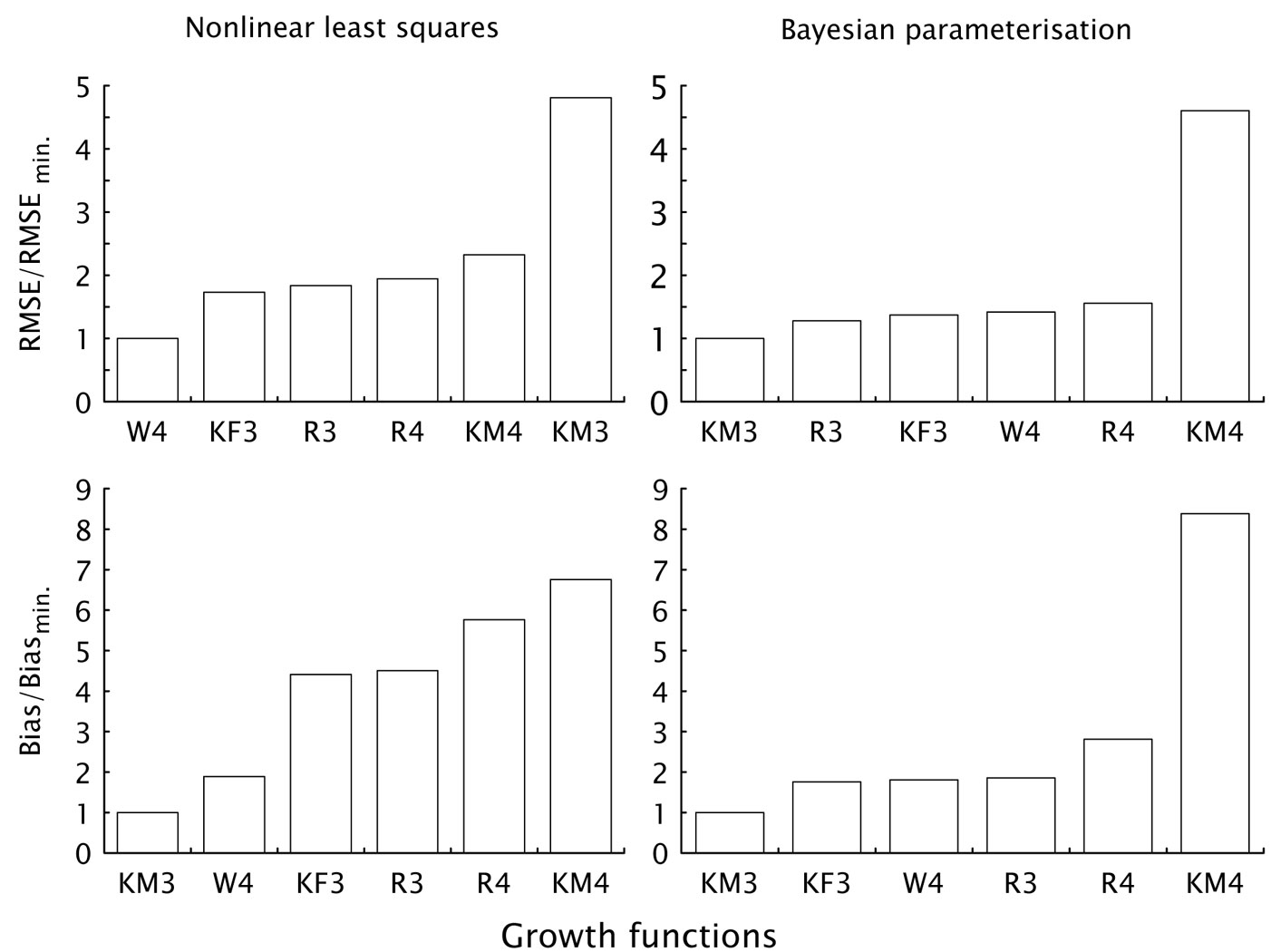
Comparing the selected growth functions across parametrization methods, the W4 function produced more robust results and smaller differences among parametrization methods. Moreover, the KM3 function can produce excellent results as far as biases are concerned. However, when using the NLS method, the small bias was offset by a significant decrease in the overall accuracy of predictions. Furthermore, the four-parameter version of the KM-function resulted among the worst functions, especially in combination with the Bayes parametrization. This evidence is exactly the opposite of that obtained from the results of three-parameter version. Similar considerations hold for the three and four-parameter versions of the Richards function. In the latter case, the three-parameter function was similarly better than the four-parameter version for both parametrization methods and modeling aims, although differences were not so pronounced.
Discussion
The most important characteristic of the KM-function is its time-determinate feature, i.e., the function predicts the complete termination of growth when the organism reaches its final size. A more detailed analysis of the integral and differential forms of the KM-function showed that:
- The integral form (eqn. 2) admits the possibility of starting the growth at the age of
t(0)=0 ,and at a given age, it simultaneously admits the possibilityy(0)=0. The differential form (eqn. 3) at the age oft(0)=0 predictsdy/dt=0; RGR at the age oft(0)=0 is not defined. However, it holds true that ift(0)→0, RGR is limited in its approach to infinite RGRmax. - The position of the inflexion point within the life cycle is not fixed. The inflexion of the growth curve can occur at any age t and value y.
- In the period of growth cessation at the time
t=tmax, the integral form (eqn. 2) predictsy=ymax, and simultaneously (eqn. 3) at the age oft=tmax it holds true thatdy/dt=0 and consequently, RGR = 0.
Property (1) is shared by Richards, Weibull and KM functions and contributed significantly to their popularity. It does not contradict the known biological laws and contributes to the feasibility of growth modeling at the early life stages. The Korf function at the age of t(0)=0 has neither the defined value y(0) nor the value dy/dt, thus the possibility for growth to start from the zero point is excluded.
From properties (2, 3) it follows that the KM-function is a model of time-determinate asymmetrical growth starting at zero size of an organism and terminating when it reaches its final size. Since the KM-function does not merely approach asymptotically, but exactly reaches both the starting and the final size, the equation assumes a finite length for the growth period of an organism. This represents an independent parameter in the equation tmax and can be satisfactorily estimated by means of the maximum age of the tree species under the particular natural conditions. Simultaneously, the age of growth rate culmination can occur at any time t ∈ [0, tmax] and at any value y, resulting in the capability of the growth function to represent any degree of time growth asymmetry.
The growth function Beta ([36]) is the only other function known from the literature which is able to describe in a continuous way the determinate growth of living organisms. It is based on the application of the frequency function of Beta distribution, which is a more general alternative to the KM-distribution. As a result, a number of common properties are shared by the Beta and the KM-function.
Yin et al. ([36]) point out the following properties of the Beta function: (i) its flexibility - the point of inflexion of the growth trajectory may occur at any position; (ii) good parametrization properties resulting from clear interpretability of parameters, and in particular (iii) the possibility to estimate the final value of yield at the end of the production period. These advantages are also true for the KM-function, especially in its three-parameter version.
Easy and stable parametrization of the three-parameter KM-function results from a good biological interpretability of parameters, likely stemming from its smaller intrinsic curvature. Indeed, the integral form of the KM-function does not contain any exponential terms (eqn. 2). Consequently, the equation is similar to Hossfeld and Levaković growth functions ([38] - eqn. 4, eqn. 5):
According to Kiviste ([14]), Zeide ([38]) reports that these equations are surprisingly accurate, though they are among the oldest growth functions known.
On the other hand, the four-parameter KM function version provided poor predictions on the dataset tested in this study. Also, the three-parameter KM function along with NLS parametrization method provided relatively large RMSE. The above facts suggest that, despite its expected small intrinsic curvature, the KM function may have a rather large parameter-effect curvature. The inclusion of an additional parameter into the KM function led to the instability in the estimation of parameters, and consequently the accuracy was notably reduced, even for short-term predictions. The same scenario hold also for the Richards’ function.
The problem of the relatively large parameter-effect curvature of the KM-function may be solved by the inclusion of biologically meaningful constraints into the process of parameter estimation. For example, fixing the parameter value tmax based on its biological interpretation (i.e., the expected lifespan of the organism considered) has proven to be useful, especially when further information on other parameters was included into the estimation process by the Bayesian estimation procedure. As a result, the three-parameters KM function was assessed as the second most successful function.
A good accuracy of the KM-function is also expected based on additional theoretical reasons. Despite several shared properties, KM and Beta functions also show some differences. The differential form of the Beta function, obtained from the original frequency function of the Beta distribution under the assumption t(0)=0 and arbitrarily fixing the parameter δ = 1, is the following ([36] - eqn. 6):
where ti is the time of growth rate culmination and c is the maximum growth rate at time ti. The above function has both expansion and restriction elements linked to age, i.e., the expansion element is a power function and the restriction element is a linear function of age. The biological rationale for the linearity of the Beta function restriction element is problematic: the problem originates from the fixation of δ in the original Beta function because of the need for analytical integrability of the eqn. 6. In the KM-function, both elements represent a power function of age, thus being theoretically better fitting to empirical data.
Linkage to t of expansion and restriction elements of the differential form is a quite rare property. The age t has both positive and negative influence on growth rate dy/dt, though the negative influence prevails increasing the age. The only other well-established function having this property is the Weibull growth function, whose differential form is as follows (eqn. 7):
Another similar growth function was proposed by Sloboda (eqn. 8):
whose expansion element is linked to the interaction of age and size. In almost all other growth functions, the expansion element is linked to size y and the restriction component to age t. Consequently, KM, Weibull and Sloboda’s functions admit the possibility of initial age t(0)=0, assuming dy/dt = 0 at this age. On the other hand, classical Weibull and Sloboda’s equations are typical representatives of non-determinate growth models, in which if t→∝, then y→ymax and dy/dt→0, i.e., they implicitly assume an infinite lifespan for the organism studied.
The KM, Beta and Weibull growth functions, along with the Richards and Korf functions, share an additional feature: all functions have y(0)=0 at the age t(0)=0, that is, they do not have a defined RGR (i.e., if t→0 then RGR→∝). Unlike the above equations, the integral form of the Sloboda’s model does not allow the possibility y=0 at any age, thus RGR is defined and equal to 0 at the age t(0)=0. Based on the above considerations, it follows that Weibull, Beta and KM functions are not suitable for modeling the exponential growth in the initial life stages (e.g., at t<1), since the classical growth analysis assumes that the growth rate is proportional to size, i.e., the final RGR approaches the final maximum value.
Comparison of the selected growth function properties proved the usefulness of the KM-function for growth modeling purposes. The three-parameter version (KM3), combined with the Bayes parametrization method, was the second most successful function for short-term predictions of tree diameter growth on the studied dataset. In particular, such model was suitable for bias minimization.
As expected, results of this study showed that the Bayesian parametrization method performs slightly better in minimizing the modeling errors. Also, NLS was slightly more suitable when minimization of biases is required in short-term predictions. However, differences in RMSE and biases among the parametrization methods used were relatively small, probably due to the fairly large number of measurements covering most of the life cycle of trees. Using high quality empirical measurements, the above differences are diminished because the importance of a priori parameter distributions quickly decreases in the Bayesian procedure ([4]).
Conclusions
The analysis carried out revealed several useful theoretical properties of the KM-function:
- good fitting to empirical data and high interpolation accuracy, due to the possibility of inflexion at any y value and the power form of both key components in the differential equation;
- realistic growth reconstruction of backward extrapolations based on empirical measures, thanks to the possibility of predicting
y(0)=0 anddy/dt= 0 at the aget(0)=0, consistently with known biological growth laws. - realistic growth predictions of forward extrapolations based on empirical measures, thanks to the a priori inclusion of a parameter related to the final length of life cycle and the final size of the organism.
Results of the comparison of the KM-function with selected classical growth functions proved its usefulness for modeling the growth in diameter of individual trees, in particular in its three-parameter form combined with Bayesian parametrization when minimization of prediction bias is needed, while the use of four-parameter Weibull function combined with the NLS parametrization method is recommended for the short-term prediction of diameter growth.
Acknowledgements
This study was supported by the European Structural Fund under the project ITMS: 26220120069 (Center of Excellence for decision support in forest and landscape at the Technical University in Zvolen, Slovakia, Activity 3.1 Experimental and methodological platform of precision forestry tools) and by the Scientific Grant Agency of the Ministry of Education, Science, Research and Sport of the Slovak Republic under the project 1/0618/12 and 1/0953/13. Additional support was received from the National Agency of Agricultural Research of the Czech Republic under the contract No. QJ1320230.
References
Gscholar
Gscholar
Gscholar
Gscholar
Gscholar
Gscholar
Gscholar
Gscholar
Gscholar
Gscholar
Gscholar
Gscholar
Gscholar
Gscholar
Authors’ Info
Authors’ Affiliation
Lubomír Scheer
Faculty of Forestry, Technical University in Zvolen, T.G. Masaryka 24, 960 53 Zvolen (Slovak Republic)
Faculty of Forestry and Wood Sciences, Czech University of Life Sciences Prague, Kamýcká 1176, 165 21 Praha 6 - Suchdol (Czech Republic)
Corresponding author
Paper Info
Citation
Sedmák R, Scheer L (2015). Properties and prediction accuracy of a sigmoid function of time-determinate growth. iForest 8: 631-637. - doi: 10.3832/ifor1243-007
Academic Editor
Renzo Motta
Paper history
Received: Jan 15, 2014
Accepted: Oct 17, 2014
First online: Jan 13, 2015
Publication Date: Oct 01, 2015
Publication Time: 2.93 months
Copyright Information
© SISEF - The Italian Society of Silviculture and Forest Ecology 2015
Open Access
This article is distributed under the terms of the Creative Commons Attribution-Non Commercial 4.0 International (https://creativecommons.org/licenses/by-nc/4.0/), which permits unrestricted use, distribution, and reproduction in any medium, provided you give appropriate credit to the original author(s) and the source, provide a link to the Creative Commons license, and indicate if changes were made.

Web Metrics
Breakdown by View Type
Article Usage
Total Article Views: 58904
(from publication date up to now)
Breakdown by View Type
HTML Page Views: 47305
Abstract Page Views: 3634
PDF Downloads: 6286
Citation/Reference Downloads: 43
XML Downloads: 1636
Web Metrics
Days since publication: 4204
Overall contacts: 58904
Avg. contacts per week: 98.08
Article Citations
Article citations are based on data periodically collected from the Clarivate Web of Science web site
(last update: Mar 2025)
Total number of cites (since 2015): 2
Average cites per year: 0.18
Publication Metrics
by Dimensions ©
Articles citing this article
List of the papers citing this article based on CrossRef Cited-by.
Related Contents
iForest Similar Articles
Research Articles
Impact of climate change on tree-ring growth of Scots pine, common beech and pedunculate oak in northeastern Germany
vol. 9, pp. 1-11 (online: 13 October 2015)
Research Articles
A comparison of models for quantifying growth and standing carbon in UK Scots pine forests
vol. 8, pp. 596-605 (online: 02 February 2015)
Research Articles
Probabilistic prediction of daily fire occurrence in the Mediterranean with readily available spatio-temporal data
vol. 10, pp. 32-40 (online: 06 October 2016)
Research Articles
Distribution factors of the epiphytic lichen Lobaria pulmonaria (L.) Hoffm. at local and regional spatial scales in the Caucasus: combining species distribution modelling and ecological niche theory
vol. 17, pp. 120-131 (online: 30 April 2024)
Research Articles
Nonlinear mixed model approaches to estimating merchantable bole volume for Pinus occidentalis
vol. 5, pp. 247-254 (online: 24 October 2012)
Research Articles
Local ecological niche modelling to provide suitability maps for 27 forest tree species in edge conditions
vol. 13, pp. 230-237 (online: 19 June 2020)
Research Articles
Incorporating management history into forest growth modelling
vol. 4, pp. 212-217 (online: 03 November 2011)
Research Articles
Spatio-temporal modelling of forest monitoring data: modelling German tree defoliation data collected between 1989 and 2015 for trend estimation and survey grid examination using GAMMs
vol. 12, pp. 338-348 (online: 05 July 2019)
Research Articles
Modeling compatible taper and stem volume of pure Scots pine stands in Northeastern Turkey
vol. 16, pp. 38-46 (online: 22 January 2023)
Research Articles
Facilitating objective forest land use decisions by site classification and tree growth modeling: a case study from Vietnam
vol. 12, pp. 542-550 (online: 17 December 2019)
iForest Database Search
Search By Author
Search By Keyword
Google Scholar Search
Citing Articles
Search By Author
Search By Keywords
PubMed Search
Search By Author
Search By Keyword


