Open field-applicable instrumental methods for structural and functional assessment of whole trees and stands
iForest - Biogeosciences and Forestry, Volume 8, Issue 3, Pages 226-278 (2015)
doi: https://doi.org/10.3832/ifor1116-008
Published: Sep 03, 2014 - Copyright © 2015 SISEF
Review Papers
Abstract
This illustrated review is aimed to provide succinct account of different methods applicable for obtaining objective information about the functional ecology of forest sites and stands (and also, e.g., orchards, watersheds, parks or alleys) for the purposes of phytotechnology or precise forestry. Management strategies must consider preservation of many important functions of forests in the landscape. Management methodologies include classical forestry approaches based on classification of the natural environment according to climatic zones, soil characteristics and composition of herbaceous as well as woody vegetation. One possibility for obtaining objective information came with the development of ecologically applicable instrumentation, allowing studies on the whole tree and stand levels to be undertaken anywhere in the field. Information may be derived at sites that are not permanently observed and are not equipped with additional constructions, such as towers, masts, or greenhouses. These field applicable methods are focused especially on tree and stand macrostructure, water relations and functional parameters of trees. In addition, problems associated with interactions between trees and different organisms are also discussed. A series of methods based on different principles is useful to measure mostly quantitative, operative or effective tree parameters as tree crowns and leaf distribution, stems (or large tree trunks) and root systems including skeleton and absorptive fine roots. This is sometimes possible to do with rather simple methods, but instrumental methods prevail especially for root studies. In addition to several classical measurement principles including anatomical or mechanical sensing, the methods work with sound speed (acoustic tomography) using electromagnetic rays of different wavelength (from radar to optical), electric conductivity or impedance, supersonic air stream and thermodynamics for example. Methods for data evaluation and examples of application are also included. The whole complex system approach should serve for different scientific fields (including hydrology, landscape care, horticulture, forensic engineering, etc.) and especially to support precise forestry.
Keywords
Instrumental and Simple Methods, Geometrical and Effective Parameters, Tree Crown, Stem (trunk) and Root System, Complex Studies, Water and Energy
Introduction [1]
Proper management of forest ecosystems from a biological perspective is dependent on classification of the natural environment for the purposes of phytotechnology (e.g., thinning operations) and forestry management. Functional management goals may include timber production as well as other important functions of forests in the landscape, such as water sources for people, but also for control of climate, maintenance of biological diversity, recreation, etc. for which importance often increases with time. Such functions have been working automatically in the past, but serious environmental impacts on forests associated with anthropogenic activities (e.g., air pollution, soil acidification) and global climatic change became apparent at the end of the 20th century.
Therefore long-term experience of foresters should be supplemented with additional objective information, which may be used to help solve new problems. This includes application of modern electronics, computers and other technologies, as well as collection of necessary data in the field especially pertaining to ecophysiology. This review provides only a brief description of methods suitable for studies at the whole tree and stand levels (and even higher levels). The methods are applicable under open forest conditions using mobile instrumentation approaches that can be used almost everywhere. They were tested in more than 60 sites and in over 50 woody species in Europe, USA and Australia. We focused on measurement and evaluation of macrostructure and water flow, because the maximum energy flow in ecosystems goes through water and water is the most frequent natural limiting factor of tree growth and functional states of whole trees and stands (if not considering polar regions and tops of high mountains). Ecologically oriented scientific fields and practically oriented field activities in forestry, arboristics, horticulture, hydrology, remote sensing and forensic engineering use many traditional and modern methods.
Annual and seasonal stem growth are probably the most frequently studied processes in forestry. Usually institutions for forest management (IFM) base their practices on this valuable data on a large scale (e.g., national), which provide crucial information about timber production and yield. A great body of literature is available on this topic. However, strategy for the management of forest ecosystems in Europe elaborated over several centuries is focused on classification of the natural environment and determining potential natural vegetation and oriented not only toward production but also on preserving other important functions of forests in the landscape. A detailed version of this approach was successfully applied for over 80 years. The eventual impact of anthropogenic activities and global climatic changes led to development of ecophysiological methods applied to evaluate the functional state and development of forest ecosystems.
These methods were usually overlooked in the past because previous technologies did not permit their application in the field and because it was supposed that they possessed limited possibilities for practical application. Fortunately, this situation is changing rapidly due to the availability of modern electronics, computers and other technologies. Additional methods are being developed and are also used for practical applications in the open field. We are not presenting a comprehensive excellent review as published recently (see [101], [14], [148], [142]). Instead, we are focusing only on providing a brief description of methods that we have actually tested under open forest conditions (mostly outside permanent research plots) and with which we have obtained good results. Use of the whole tree and stand approach in addition to mobile instrumentation that can be used almost everywhere are prerequisites for this purpose.
This overview is aimed to assist studies at the whole tree and stand levels that are applicable under any field conditions and for various purposes. It provides a broad source of information including (traditionally spoken) specific fields such as different parts of tree structure (e.g., individual leaves or root tips). The reader can select the parts, which he may actually need, but keep in mind, that we always analyze whole organisms, and no individual component can represent a living object. A series of very simple and more complicated instrumental methods that are applicable in field studies are described together with methods for interpreting the results. In this presentation, details were avoided, thereby allowing the text to be substantially shortened (to approximately one paragraph per method); for details, please see the cited literature sources. We also respected the fact that figures provide large amounts of information in a small space. Therefore, 59 complex figures (over 160 individual figures) are presented. Overviews such as this can never be exhaustive, because old methods are gradually abandoned and new methods are continually developed or improved. The application of similar methods is a fundamental step towards more qualified management of forest stands, which is the principle of Precision Forestry, as well as a better quantitative understanding of hydrological and ecological processes in forest enterprises as well as natural forests, and a factual foundation required for accurate decision making in forensic engineering.
Classical forestry practices [2]
Forest management and planning
Forest management strategy in Europe has been based on complex planning documents i.e., forest management plans developed over a period of more than 60 years particularly in the Czech Republic ([118], [188], [189], [130]). Such plans are elaborated for planning periods of 10 years and deal with the details of management of all forest stands within particular forest enterprises, taking into account age, species composition and stand structure (Fig. 1, Fig. 2). These background factors are considered according to the aim of the management and are estimated based on the amount and quality of natural production and protection of water sources (and other benefits from forests, such as recreation), particularly from the viewpoint of sustainable forest management. Special management of natural (virgin) forests (Fig. 3) is also included. Forest management plan is composed of text, graphics (forest maps) and stand records that describe the individual forest stands and the proposals of the forestry measures (Fig. 4).
Fig. 1 - An example of a forest stand with natural species composition (oak 60%, ash 40%, elm interspersed) in a floodplain forest along the Morava River, Czech Republic (upper panel). The site belongs to the 1st forest vegetation grade (elevation of 195 m above sea level) and to oak (Quercetum) forest altitudinal vegetation zone. It is in the category of nutrient rich soils with a big storage of humus, often gleyish and waterlogged with frequent local spring floods. Natural-like mostly beech forests “Voderadské bučiny” (Fagetum), Jevany region, Central Bohemia, with a sparse herbaceous layer beneath dense crowns and higher plant density at the edge of such forests (lower panel).
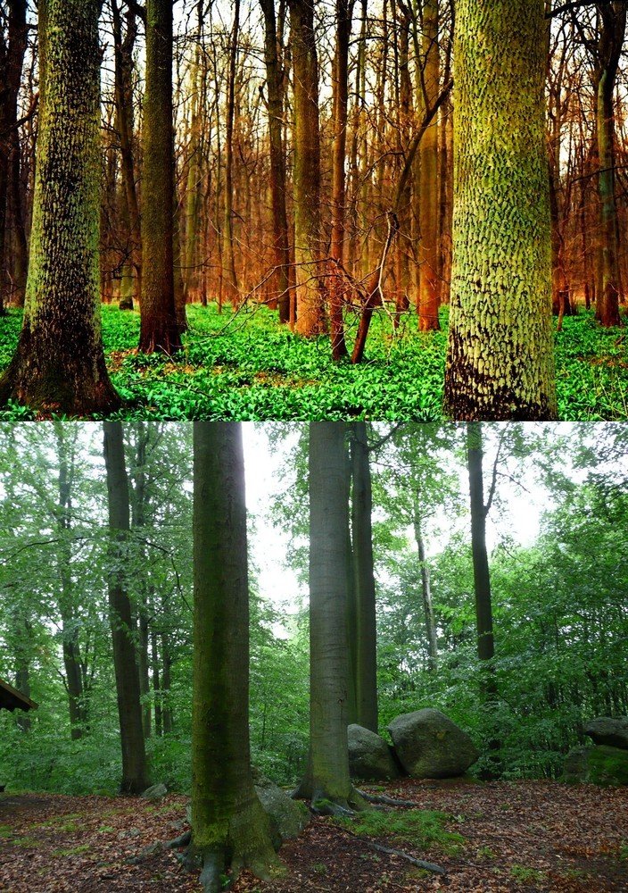
Fig. 2 - Example of a forest stand with unsuitable species composition (Norway spruce 100%) at a nutrition rich site in the framework of 3rd vegetation altitudinal zone (Querceto-fagetum), altitude 400 m (upper panel). Closed canopy spruce forest stands are causing increased acidity of soils (due to needle litter) and reduce development of herbaceous layers because of light limitation. Young and medium age spruce forests themselves (with usually maximum LAI at that phase of their life) often suffer drought and are very vulnerable to bark-beetle attack. The national natural reserve in Bíla Voda, Jeseníky Mountains, Czech Republic is a different situation. Natural-like forests managed by “controlled decay” system are very resistant and bark beetles cause minimum damage (photo: R. Mrkva 2012 - lower panel).
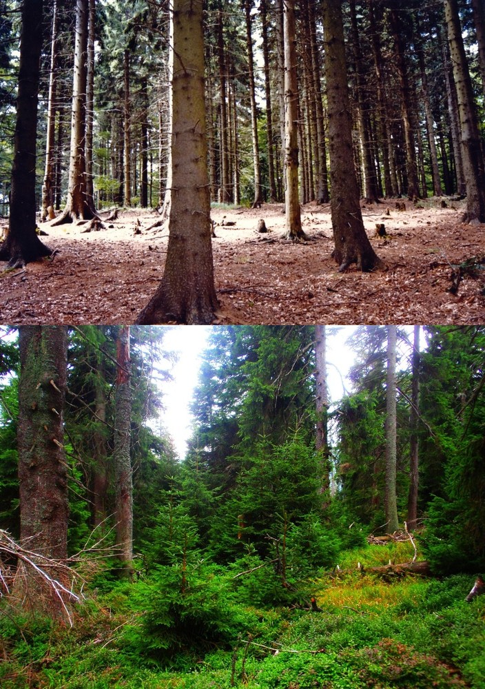
Fig. 3 - Contrasting virgin forests in very distant parts of Europe: mountains in Canary Islands (Gomera - upper panel) with dense forests composed of many (up to about 30), woody species, but prevailing Laurus azorica, Myrica faya and Persea indica. Virgin forests in northern Lapland (Finland) at the tree line in the mountains. The forests on the flat hilltop are dominated by Pinus sylvestris and in the foothills dominated by the same species and Picea abies (Varrio - middle and lower panels).
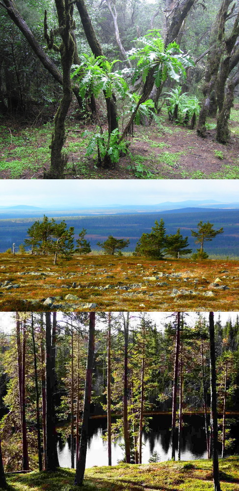
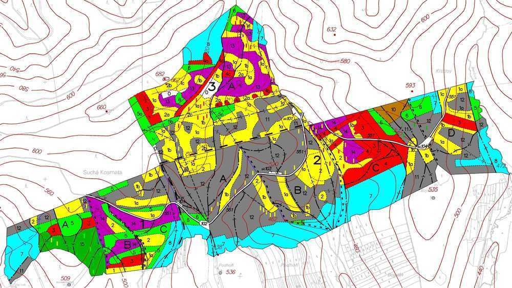
Fig. 4 - Examples of forest maps characterizing particular forest stands and site characteristics classification suitable for management purposes including selection of representative experimental sites / stands, if any new study should be done there. Common forest stand maps show characteristics of different stands, their age and species, usually at the scale 1:10000. Letters and numbers mark individual stands. Colors indicate age classes per 20 years each: white = clear area, yellow = 1-20 years, red = 21-40, green = 41-60, blue = 61-80, brown = 81-100, gray = 101-120. Hatching marks stand density. Forest roads are marked according their quality. Forest units are marked in three functional levels for orientation, integration and management.
Typological system (classification) of forest management
In Europe, the typological system of forest management historically involves a complex description of environmentally defined units. Because there was almost no instrumental technology available in the past, these descriptions were based on careful observations (descriptions of plant communities, climatic data, terrain conditions and soils) as well as practical experience. The climatic description begins first with a determination of vegetation altitudinal zones, which reflect temperature (or preferably, evaporation power, which depends to a large extent on radiant energy load) and precipitation gradients and their impact on phenology and growing conditions (Tab. 1). Terrestrial ecosystems respond to global climate change in the landscape at regional scales ([238]). To ensure a practical application of geobiocenology, vegetation zones are delimited using bioindicators based on the occurrence of characteristic plant species and their communities (Fig. 5). Forest biotopes are then defined in a more detailed way based on dominant site conditions, including soil conditions and orography and distinguishing acid, fertile, enriched by water and humus, gleyish waterlogged and extreme soils (Fig. 6). Local specialists modified details of this approach ([26], [27], [111], [112], [105], [187], [247], [246], [192], [154], [16], [19], [20], [232]). Similar typological systems for forest management were adopted in the United States ([75], [239]), Russia ([218]), Canada ([124], [125], [112]), India and Burma ([72]) and Socotra, Yemen ([87], [86]). This widespread adoption is evidence that the principles of this approach are sound (see also [81]) and can be applied anywhere in the world. An example of a typological map characterizing the forest stands (see Fig. 1 to Fig. 2) is presented in Fig. 7. Specific typological systems are compatible (and eventually transformable) to similar typological systems applied in other countries ([234], [74]).
Tab. 1 - Range of climatic parameters characterizing forest altitudinal vegetation zones.
| No | Forest altitudinal vegetation zone |
Altitude [m] |
Mean annual temperature [°C] |
Mean annual precipitation total [mm] |
Length of growing season, days with temperature above + 100 °C |
|---|---|---|---|---|---|
| 0 | Pine | - | - | - | - |
| 1 | Oak | Below 350 | Above 8.0 | Below 600 | Above 165 |
| 2 | Beech-Oak | 350-400 | 7.5-8.0 | 600-700 | 150-165 |
| 3 | Oak-Beech | 400-550 | 6.5-7.5 | 650-800 | 150-160 |
| 4 | Beech | 550-600 | 6.0-6.5 | 700-900 | 130-150 |
| 5 | Fir-Beech | 600-700 | 5.5-6.0 | 750-900 | 130-140 |
| 6 | Spruce-Fir-Beech | 700-900 | 4.5-5.5 | 900-1200 | 100-130 |
| 7 | Beech-Spruce | 900-1050 | 4.0-4.5 | 1100-1300 | 100-120 |
| 8 | Spruce | 1050-1350 | 2.5-4.0 | 1200-1500 | 60-100 |
| 9 | Dwarf pine | 1350-1600 | Below 2.5 | Above1500 | Below 60 |
Fig. 5 - Scheme and hierarchy of main elements of the natural environment - forest types.
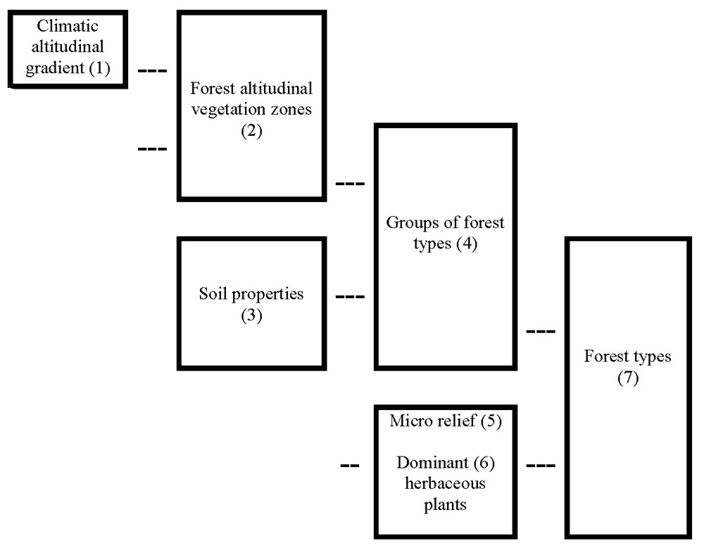
Fig. 6 - Differentiated forest management systems within the ecological network of forest types (Simon 2014, unpublished).
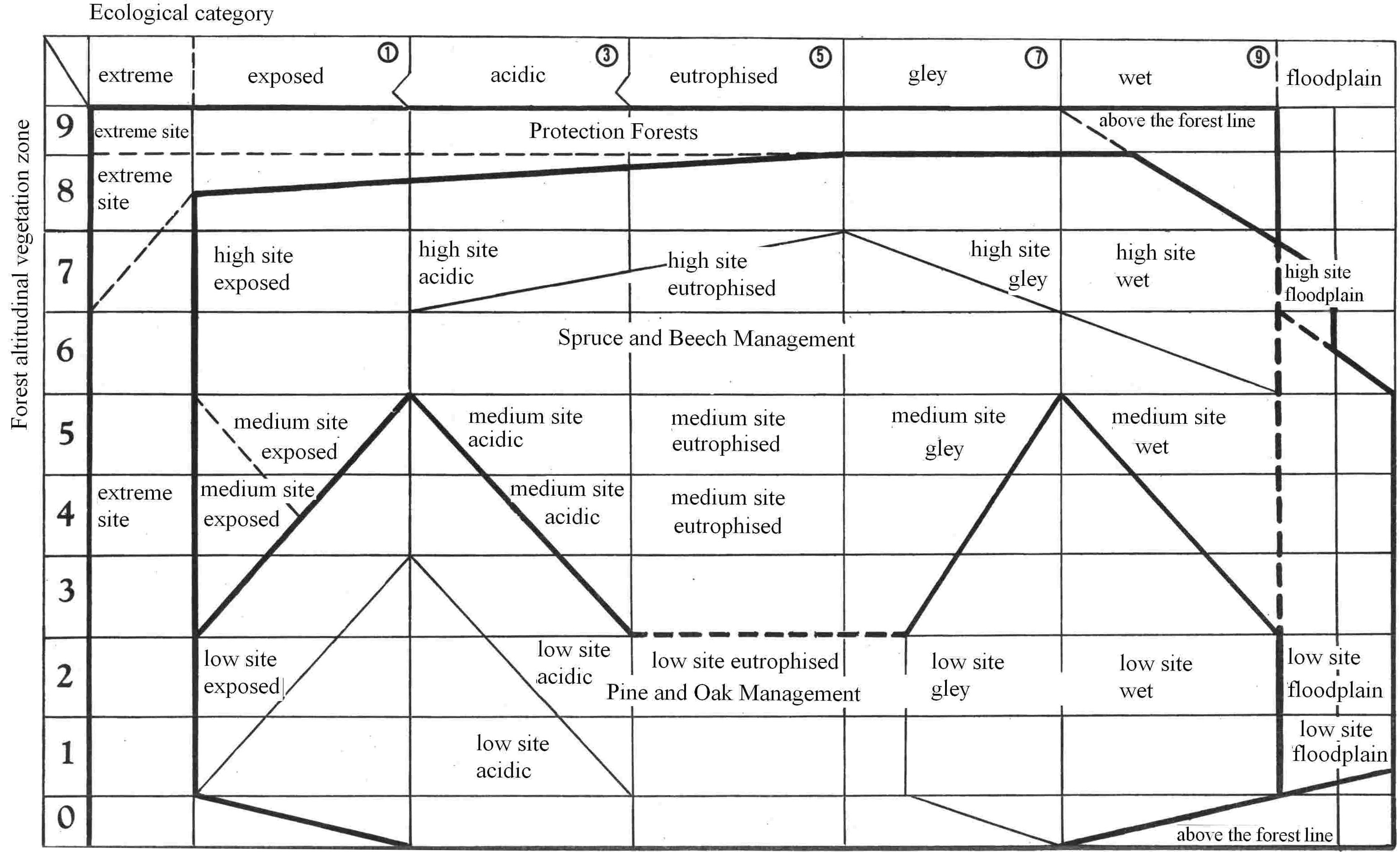
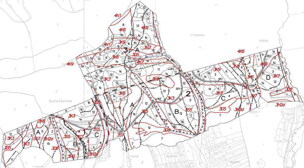
Fig. 7 - Forest typological map characterizing forest types, i.e., segments of the potential natural vegetation. In addition to marked stands, red letters and numbers characterize abbreviations of individual forest types. Ecological characteristics include soil parameters and available soil water: extreme, acidic, nutrient-rich, enriched by water or humus, gleyish, waterlogged. Micro relief patterns are marked in extreme cases, e.g., nurseries, loess, cutting slopes along rivers, etc. This map serves as a background for management differentiation and proper selection of forestry technologies.
When the above systems are related to energy and water flow, a rather simple model relating the vegetation altitudinal zone conditions, which are expressed as the ratio of the annual total of precipitation (in millimeters) to the mean annual temperature (°C, the simple classical Lang’s rain factor), can be developed. This model, which allows us to describe the actual condition and predict the future development of forest types in the entire Czech Republic, was expressed in a series of maps ([116], [15], [17], [18]). Previous ecological forecasts based on the predicted consequences of global warming have usually proven to be true.
Biometrical analysis of stands - forest inventory
Forest inventory typically focuses on forest stands (as well as on species and sometimes even on individual trees, particularly in mixed stands) and estimates of forest development from the viewpoint of desirable and non-desirable targets and the application of silvicultural practices. This type of inventory provides the fundamental background necessary for mathematical modeling and planning ([126], [210], [190], [82]). Specific targets of forest management plans, particularly those focused on forest regeneration and silvicultural practices (including allowable cutting, logging cost, sustained and prescribed yield and target diameter felling), are defined. The effectiveness of forest management plans is assessed according to operative evidence of forest inventory ([216]).
Modification of forest management
Most of the technologically oriented approaches that were applied in the past in the old Austrian empire, including many Central European countries as well as the present Czech Republic, have been changed during recent years due to global climatic changes, particularly local drought. As a result, more detailed information about the present and future behavior of forests, particularly in terms of energy and water relations, mineral supply, background for physiological and mechanical stability and other factors, is required for decision-making. This information can be provided through ecophysiological studies, which represent additional instruments for planning activities. These studies provide an additional, integrative approach to forest evaluation that can be combined with classical forest inventory searches. A variety of biometric methods based on rich empirical experience and on mathematical models derived from this experience have been used for this purpose ([7], [84], [211], [190], [207]). The present contribution aims to briefly describe some movable field-applicable methods that have already been verified at over 60 forest sites or orchards and for over 50 woody species from northern Lapland through the Canary Islands (see Fig. 3) and both US coasts to southern Australia and to provide examples of their application. The application of the findings of these studies permits the optimization of forest management measures under changing environmental conditions, even under conditions of changing economic strategies ([71], [207]).
Precision forestry - functional ecology approach
Fundamental terms and problems [3]
Macrostructure, water and energy in ecosystems
Ecosystems possess many measurable biometric as well as physiological parameters. These parameters include the balance of energy, water, carbon, mineral elements and others. Quantitatively, water and energy balance are usually 1, 2 or 3 orders of magnitude larger than the balances of other elements. However, other elements are also important; in fact, their importance is greater in terms of the information included in ecosystems. Nevertheless, it should be kept in mind that water and energy serve as the necessary basis for any living (eco-physiological) system and, consequently, for all living processes. Water and energy cannot be neglected if any other features of tree behavior are to be studied. Although all life on Earth is based on the flow of radiant energy from the Sun, the Earth’s temperature must be kept within necessary limits, and water plays a crucial role in this regulation ([229], [208], [13], [182], [129], [155]). When the energy flow is too high, an increase in the surface temperature above the acceptable upper limit occurs. Plants can survive only when their exposed parts, leaves, which are needed to absorb radiant energy, are effectively acclimatized, i.e., cooled. The largest amount of water required by plants is used in cooling (associated with the heat of vaporization); only minor amounts of water (less than 1%) are used in all other processes, including the transport of assimilates and growth. Forests represent the largest control mechanism of the Earth’s water cycle and climate up to the continental level ([141], [138], [139]). This problem is also associated with occurrence of hurricanes ([140]). If frosty regions in polar areas and the tops of high mountains are not considered, water is the most frequently limiting factor for plant growth.
Example of unfavorable climatological situation in regional scales
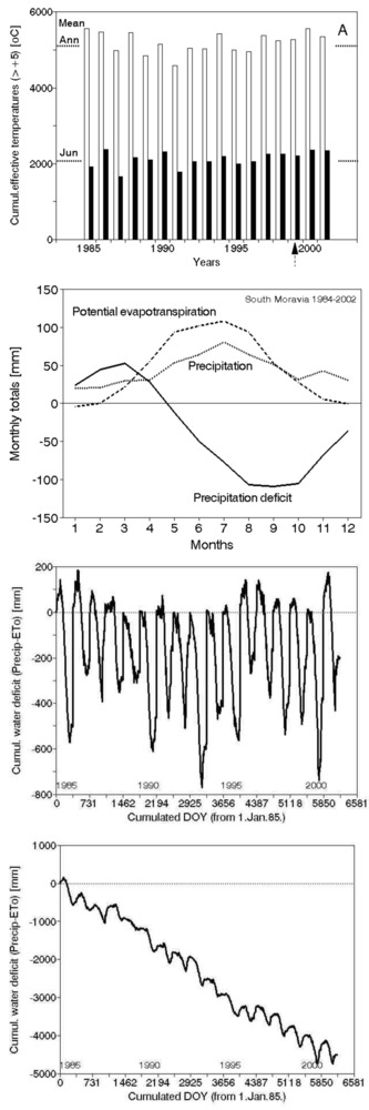
An example given in Fig. 8 shows the climatic situation in one region of Central Europe (southern Moravia), in particular. No clear differences between two years can be distinguished easily on the basis of individual meteorological parameters only. However the complex parameter as the precipitation deficit (precipitation minus potential evapotranspiration) Σ (P-PET) cumulated over the growing season clearly shows differences between two compared years ([9], [10], [1]). The annual and monthly totals of effective air temperatures exhibit practically no increase over almost 20 years (Fig. 9, top panel). The meaning of the precipitation deficit is similar to that of Lang’s factor, but it is physically much sounder (it characterizes simplified water balance that does not include soil water content and flows). The values of the precipitation deficit are shown over the mean growing season (Fig. 9, second panel), as annual courses during the years 1985 to 2002 (Fig. 9, third panel) and as cumulative annual values (Fig. 9, fourth panel). Especially the last panel demonstrates that, during the mentioned period of time, almost 5 m of water (approximately 250 mm each year) is missing. Therefore, lack of water is the main trend for the region. This situation here and correspondingly also in other regions naturally also has its phenological consequences ([174]). Although this simple calculation provides only approximate values, it indicates that problems with water are increasing and could have a serious impact in the near future. Water problems definitely cannot be neglected. Even politicians, who organized a meeting of ministers focused on the topic “Water as the strategic commodity and possibly the largest problem in international politics in Cyprus in the future, recognized these problems” in Cyprus (October 2012). Tree structure mostly reflects adaptation to energy and water relations. The water conducting system of trees, which includes xylem and phloem, represents the largest volume fraction of trees and stands. Tree growth and forest production are nothing else other than changes in that volume and mass. Fortunately, tree water relations can be measured rather easily with presently available methods and instrumentation.
Fig. 8 - How to understand meteorological (or climatic) data. Common meteorological data (especially for longer periods of time, such as week or month) are usually easily available at each meteorological station (monthly or daily means or totals are shown here). This includes mean total global radiation (Rg in MJ m-2 d-1), mean air temperature and sum of effective daily temperatures (above 5 °C), monthly precipitation (mm) and potential evapotranspiration (Ep in mm) calculated by Penman-Monteith or (less precisely and only for daytime by Turc’s equation).
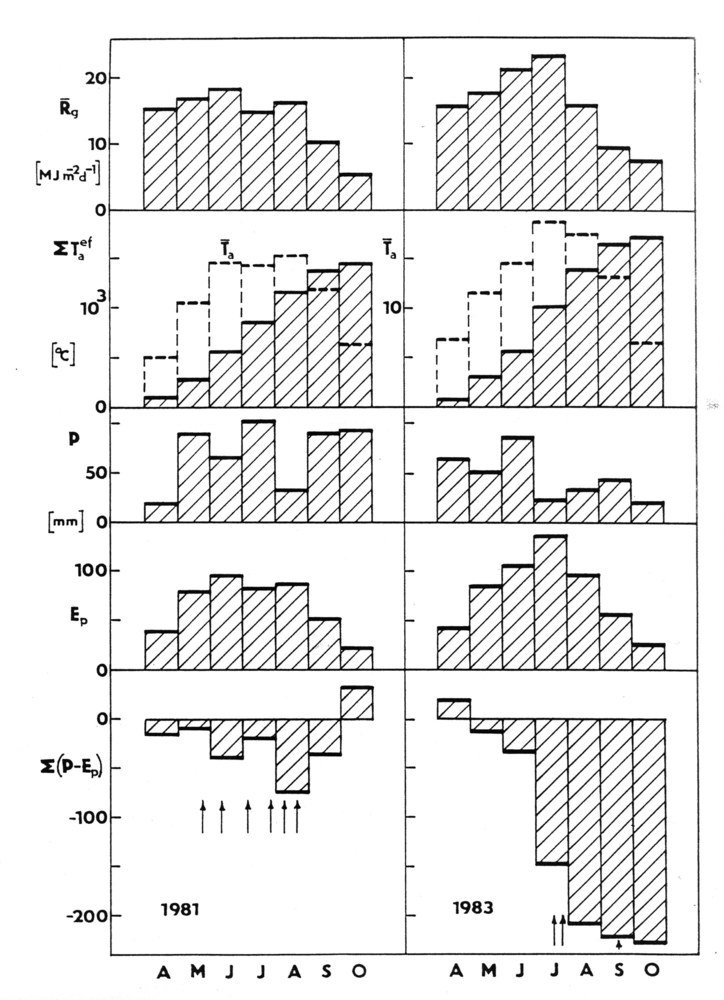
Fig. 9 - Importance of water in forest ecosystems through the example of a warmer region in Central Europe (Znojemsko in southern Moravia). Effective temperatures (> +5° C) are shown from a period of almost 20 years (data from 1985 to 2002, first panel from top). The seasonal course of mean precipitation values (P), potential evapotranspiration (PET) and the difference as precipitation deficit (P-PET) second panel) are also shown. The annual course of deficit (third panel) and cumulative precipitation deficit over the whole analyzed period of time are displayed below(fourth panel - data from HMU, [9], [10])
Jeopardizing situation with water for vegetation
Very recently, increasingly chaotic weather has been observed worldwide. Sometimes, too much precipitation and resultant flooding occur; at other times, serious drought brings higher air temperatures, limited yield, and occurrence of fires and gradual destruction of the landscape. In the past, many ancient civilizations ended due to such changes. Temperature increases when the landscape is not adequately cooled by transpiration of vegetation, which in turn is dependent on a sufficient water supply in the form of precipitation. The water cycle is extremely important for all kinds of life, and forests represent the largest almost permanently foliaged vegetation (particularly tropical “rain forests” and boreal regions containing coniferous species) or, at least, vegetation that is foliaged over long periods of the growing season (broadleaved species). We should not forget that even in Central Europe, there are hundred-meter-deep sandy dunes, indicating the presence of deserts in this region. Forests transpire large amounts of water; water vapor condenses in the higher atmosphere and returns as rain in the small water cycle. However, 120 000 km2 of forests have been destroyed on continents every year, and 50 000 km2 of landscape have been converted to impermeable and therefore overheating surfaces. Landscape canalization, which returns liquid water to the sea as fast as possible instead of allowing it to evaporate, is one of the worst landscape management practices. In this way, the continents are losing over 500 billion cubic meters of fresh water annually. Therefore, the climatic importance of forests has become increasingly important, gradually overshadowing all other benefits (including timber production) that forests provide to human society. To achieve the aim of preserving the water balance of living forests through forestry practices, we need to better understand especially tree-water relations.
Tree macrostructure
Operative biometric parameters [4]
Operative biometric parameters in general
The very brief theoretical analysis presented above represents a sound approach to water relations processes; this approach can be used for stationary and well-equipped experimental sites for which all parameters can be determined. However, in open-field and non-equipped forests where only mobile equipment is available; the determination of all parameters is usually not possible. In these cases, practically determinable approximate values of parameters must be used, or the parameters must be replaced by other values that are available at the given site. Fortunately, the current rapid development of measurement technology often allows the field application of parameters that were only rarely used previously, even at well-equipped experimental sites. Therefore, we are rather optimistic when considering the near future, specifically, in consideration of the availability of remotely sensed data (Fig. 10, upper panel), which is available more and more frequently. They provide a huge amount of information, but require specific elaboration described in plenty of specialized literature sources. This can be only welcome, but it is not included here, where we focus on ground-based measurements. Here, we have attempted to describe briefly (roughly - one paragraph for each method or its data evaluation and/or interpretation) simply how we can apply these techniques in fieldwork, providing references to the corresponding literature when particular details are needed.
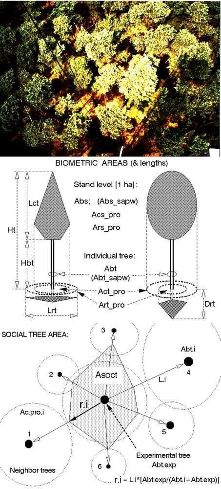
Fig. 10 - Example of the pine canopy with visible tree crowns and gaps between them (upper panel). Field measurable simple biometrical areas (using only very simple instruments, such as the tape etc.) are represented. These include: basal area (Abas), crown projected (ground plan) area (Ac_pro), eventual root projected area, (Ar_pro,), ratio of tree to stand basal area, i.e., fraction of stand basal area “belonging” to a particular tree (Ab_rat), calculated according the ratio of the tree basal area (Abas_tree) to the stand basal area (Abas_stand - middle panel). Scheme characterizing estimates of social tree area (Asoc) of the experimental tree (lower panel). Field measurements include only distances Li between the exerimental tree (marked) and all its neighbors (here shown 6 trees) and the basal areas Ab.i of all considered trees.
The simple biometric parameters
Historically speaking, a series of simple or slightly complex parameters have been applied in the early forest production-oriented literature ([123], [7], [117], [118], [184]). They all were based on tree macrostructure, presumably stems, although other parts such as the crown (with branches plus foliage) and roots (skeleton and absorptive) belong here too. Other biometric parameters, including allometric relationships, can be measured or derived in a more complicated way. A better picture of the macrostructure of a given tree or stand can be obtained by considering several simple parameters together. The basic biometric parameters are measurable with very simple instruments and often useful even for more complex measurements. They may become especially important in countries with limited infrastructure or when some sophisticated instrumentation fails in remote sites for technical reasons. These parameters include basal area (Abas), projected crown area (Ac_pro), projected root area (Ar_pro), tree height and crown base height (Ht, Hb) and crown length (CL) and width (Cw), all with additional detailed specifications (Fig. 10, middle panel). Here, we can also include some terrestrial tree areas, such as the fraction of stand basal area “belonging” to a particular tree (Ab_frac.i m2 tree-1), calculated (eqn. 4) from the individual tree basal area (Ab_tree_i) and the stand basal area (Ab_stand; total stand area, Astand is taken as 10 000 m2). Other parameters, such as timber volume or leaf area, can be used in a similar way. Summarizing all Ab_frac.i, we naturally obtain 1 ha (eqn. 1):
Another terrestrial area is the social tree area. Fig. 10 (lower panel) shows a scheme for characterizing the estimate of social tree area of a sample tree, Asoc_i, expressed in square meter per tree. The field measurements include only the distances Li between the sample tree and each of its neighbors (here, only 6 neighbor trees are shown) and the basal areas, Abas.i, of all considered neighbor trees. The social area is represented by polygon or a circle calculated from the social area radius ri according to the equation given below. Ac is additionally measured projected crown area (eqn. 2):
where ri is the “radius” of the polygon facing a particular neighbor tree (i), Li is the distance between the sample and particular neighbor trees and Ab is the basal area of the sample (samp) and neighbor trees (i). Social tree area can be also calculated by taking the mean value of ri (social position of trees) and it is more important for trees with dense crowns (e.g., spruce) than those with sparse crowns (e.g., pine).
Whole tree approach
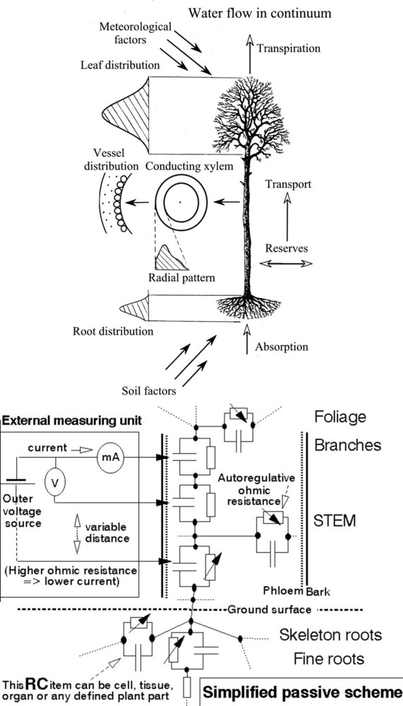
Historical forest studies were based on field measurements of tree stems, which are easily accessible and integrate the tree’s entire behavior. Such measurements include easily available macroscopic forestry inventory data. These data can be eventually complemented by additional biometrical data and eventually even with data obtained at the microscopic level (e.g., information on vessel distribution). Physiological data include relatively easily measurable variables such as tissue water content, water potential, water capacity, water storage and other parameters. However, the technology for measuring some parameters is not yet sufficiently developed to be applicable to open-field whole tree studies under the usual field conditions when no additional constructions for tree measurement are accessible. Unfortunately, methods and instruments for the measurement of whole tree carbon metabolism, including photosynthesis and respiration, and the metabolism of other elements are even less well developed. Fortunately, the situation is changing rapidly, and increasingly more instruments are becoming field- and whole-tree applicable (see e.g., ⇒ EMS Brno, Czech Republic; ⇒ ICT International, Armidale, Australia). Nevertheless, in presenting this brief review of currently available, mobile field-applicable methods, we have attempted to describe only methods and instrumentation that are robust, relatively easy to use and that we have tested successfully and with which we have obtained sufficient experience. Some structural and functional parameters applicable at the whole-tree level are illustrated in the scheme provided in Fig. 11 (upper panel), which shows that water travels in a continuum from soil to absorptive roots, conducting roots, stem sapwood, branches, shoots and foliage to the atmosphere. The same object can also be evaluated from quite different viewpoints, e.g., look at the tree as at the simplified electric circuit (Fig. 11, lower panel - Zdenek Stanek, personal communication). A tree as a whole or any part of the tree can be described by the Autoregulative Ohmic Resistance/Capacitance (RC) item. This scheme representing a non-traditional view of the system (for biologists, although it is widely used in electronics), which allows better quantification of some its properties, allows easier functional detection of feedbacks, etc. It can be applied in addition to traditional schemes.
Fig. 11 - General scheme of the whole tree underlining features measurable at this level of biological organization as well as higher ones when properly integrated (upper panel). Simplified electric circuit of the same tree (passive variant: not considering current/voltage generated by cells themselves), but indicating the position of the external measuring circuit (Zdenek Stanek, personal communication - lower panel). The external measuring circuit shows the possibilities of application of classical electronic devices working with variable electrodes geometry and related resistances of tree tissues as a background for further studies. The resistance / capacitance (RC) unit (including auto regulative ohmic resistance marked by a small arrow) can be applied to characterize individual cells, tissues, organs or any defined plant parts or the whole plant.
Tree crowns and leaf distribution [5]
Optical methods for leaf area estimates
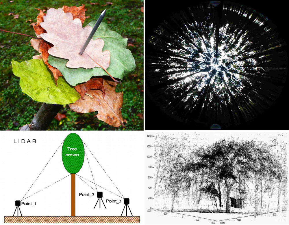
Foliage represents the fundamental organ for absorption of solar energy and the production of assimilates during photosynthesis. Therefore, if reasonable results are to be obtained for entire stands and used in further calculations, foliage should be quantified in whole tree studies. Collecting of litter by different ways is the most simple, but for broadleaved species still valid method (Fig. 12, upper panel). Optical sensors (e.g., Licor systems, fish eye) that are presently often used for this purpose are usually calibrated to provide a leaf area index (LAI in m2 m-2 or, more precisely, plant area index), including shade by branches. A fish-eye image that adequately characterizes the illumination of small plants forming the undergrowth but does not provide much information about the leaf distribution of trees within the canopy is shown in (Fig. 12, middle panel). Three-dimensional images of leafed tree crowns with a precision of approximately 5 cm can be obtained by laser scanning from a minimum of 3 stem sides (Fig. 12, two lower panels - [233]); however, this approach is applicable only to solitary growing trees (e.g., in orchards) or to trees growing in sparse forest stands where the crowns are not mutually shaded. Similar methods have also been applied in studies of entire stands using remotely sensed data.
Fig. 12 - Litter collecting is probably the oldest and most simple method for LAI measurement (5 leaves per stab, LAI= 5; several hundred stabs should be done to get a reliable mean - left upper panel). Only the seemingly small tree crowns are visible in the fish-eye image of part of the Norway spruce stand, (right upper panel). The image provides good information about the illumination of the undergrowth (the software allows modeling of any day of the year and any hour of the day if necessary), but it is also not suitable to evaluate leaf distribution in the crowns. A lidar (laser-scanning) system for evaluation of a sample tree growing in a sparse forest (where each tree was growing almost as in solitary), is set up so that the minimum of three observation points needed for spatial leaf distribution estimation with precision of 5 cm may be obtained (left lower panel). The final image is taken from one side, as applied e.g., by [233] (right lower panel).
Leaf (needle) distribution in crowns
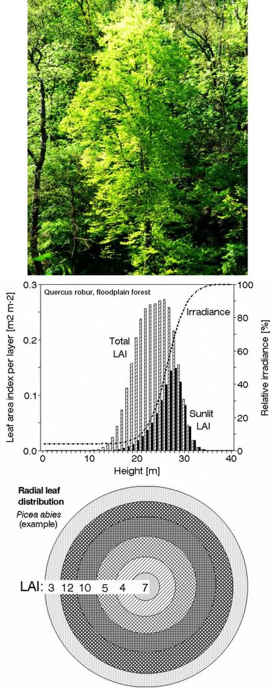
Tree crowns are very complex and difficult to describe in geometrical terms, therefore a series of methods was developed for their measurement ([108], [223]). This is especially important when considering the short-term dynamics of leaf irradiation (Fig. 13, upper panel). Classical destructive methods provide allometric relationships ([240]), allowing their wider and statistically valid use, see examples of such relationships suitable to describe vertical leaf distribution in 9 coniferous and broadleaved tree species (Tab. 2). Earlier “harvesting” methods for leaf distribution studies are much more laborious than optical methods, in which a series of sample trees are analyzed branch by branch with their exact 3D positions and corresponding leaf areas. However, because the earlier-used methods are simple and do not require expensive instrumentation (e.g., one of the most simple but well applicable methods is the litter collection - [175], [102], [191]). Similar easily applicable methods are especially useful e.g., in developing countries. The harvesting methods give more information, such as distinguishing sunlit and shaded leaf areas and vertical and radial leaf distribution in canopy layers of different depths (e.g., 0.2 to 1.0 m) and a more static view of irradiance when considering longer time periods. Fortunately, allometric equations based on such data are available for several tens of broadleaf as well as coniferous species at the level of individual trees and forest stands measured in different European countries ([235], [236], [237], [150], [151], [45], [47], [32], [59], [225], [230], [213]); these data can serve within their statistical limits until better instrumental methods are developed (Fig. 13, middle panel). The value of LAI reaches approximately 3 in pine forests, 3 to 5 in oak forests and understory cherry trees, approximately 8 in laurel forest and 7 to 12 in spruce forests. In sparse forests or orchards, we should consider 2 LAIs: the LAI for the whole stand (including gaps and reaching about 1 in an olive orchard) and the LAI for the projected crown area, e.g., 3.5 in the same orchard. These measurements are with reference to conditions in which the radial LAI within the crown reaches 1 to 7 at mid-crown and close to its outer edge, respectively). It is possible to use similar biometric methods in combination with photo images to study vertical and horizontal leaf area ([65]). Radial (or “crown cross-section”) leaf distribution may be very important for the correct interpretation of results when evaluating remotely sensed images (Fig. 13, lower panel). Similar methods can be also applied to shrubs, as it has been shown, e.g., for rhododendron ([163]).
Fig. 13 - Broadleaf tree crown in a closed canopy stand: sunlit and shaded foliage is visible (upper panel). Vertical leaf distribution (derived from allometric relationships) of total leaf area index and sunlit leaf area index (LAI, in 1m deep canopy layers) in a pedunculate oak stand and relative irradiance (Ir in percentage of that above crowns - middle panel). Solar LAI = Ir·Total LAI - in a mixed forest at the level of the entire stand (1 ha), where LAI=5 and solar LAI=1.2. Radial leaf (LAI) distribution in a single Norway spruce tree (as if all needles would fall down into individual projected crown annuli) - see large differences in LAI between individual annuli within the same crown (lower panel).
Tab. 2 - Examples of some allometric relationships for approximating of vertical distribution of leaf dry mass (in kg per defined depths of canopy layers, x [m]) or leaf area [m2] in trees from their forestry inventory data. If not calculated directly, the corresponding leaf area for each layer is derived when dividing dry mass [kg] by separately measured dry mass per area [kg m-2].
| Picea abies | canopy layer 0.5 m deep, age 40-80 years, 4 sites, x = Height H [m], y=[kg m-1]. Main eq.: y = {a exp[-b(x-c)2]+d exp[-e(x-f)2]}-g; x= DBH, D[cm]; H [m], Crown length, L[m]. Individual parameters: a=0.0145 D1.3869 ; c=0.5138 H1.1213 ; b=1.5219 e-2484 L; (orig., unpublished) d=0.0415 D1.0307; f=0.6323 H1.1008; e=1.5155 e-2027 L; |
| Pinus sylvestris | Belgium sandy area near river, age 80 years. Main equation (Rayleigh): y = {[a (htop-hi)]/b}exp {[-( htop-hi)c] d; (where hi and htop are particular height i and top height in m). x= DBH [cm]. For needle dry mass: y=[kg 0.2m-1]; a=0.003023-0.21855 x+6.065 x2; b=3.53-0.013 x; c=2.51-0.0018 x; d=0.017033+0.14593x-6.0495 x2; For needle area: y=[m2 0.2m-1]; a=0.00455-0.2952 x+10.252 x2; b=1.81 (constant)x; c=2.1 (constant) x; d=0.06143-8.448x; ([59]) |
| Quercus robur | floodplain forest, age 100 years, Main eq. to derive leaf DM per 1 m canopy depth (x1=Height [m]): y={a exp[-(x1-b)2/c]+ d exp[-(x1-e)2/f]}; x=Abas[cm2], leaf dry mass: y=[kg m-1]; a=0.0003 x1.094; b={20.89/[1+121.85 exp(-0.0116 x)]}+0.0012 x; c={21.6/[1+5 exp(-0.0042 x)]}; d=5.6E-05 x1.402; e={25.52/[1+7.182 exp(-0.0069 x)]}+0.0013 x; f=61-{53.8/[1+4.013 exp(-0.0051 x)]}; ([47]) |
| Quercus pubescens | hills in Tuscany, age 80 years, Main equation: y={a exp[-b(x-c)2]+d exp[-e(x-f) 2]}-g; here x=height [m] and y=leaf area per canopy layer [m2 m-1]. Additional equations x=DBH[cm]. a=-0.0001x3+0.0238 x2-0.826 x+13.24; b=0.4+0.62 exp(-0.9 x); c=10 exp[-2 exp(-0.046 x)]; d=0.0002 x3-0.0146 x2+0.439 x+2.68; e=-7E-0.6 x3+0.0009 x2 -0.0329 x+0.473; f=-1E-0.5 x3-0.0114 x2+1.368 x-9.351; g=0.7+0.118 x; ([67]) |
| Quercus cerris | hills in Tuscany, age 80 years. Main equation is same as above, additional equations: a=-0.0002 x3+0.0411 x2-1.614 x+24.48;_b=3E-06 x3- 0.0004 x2+0.0137 x-0.0641;_c=-0.0003 x3+0.0249 x2-0.265 x+8.64; d=2.7+0.0035 x2.1; e=0.7 exp[-2 exp(0.06 x)]; f=0.7 exp[-2 exp(-0.06 x)]; g=1.91+0.118 x; ([67]) |
| Fraxinus excelsior | floodplain forest, southern Moravia, 100 years, x1=Height [m] eq. see Q. robur; x=Abas [cm2], y=[kg m-1]; a=0.0001 x1.19; b={22.5/[1+264 exp (-0.0135x)]}+0.0003x; c={26.5/[1.45*exp(-0.0041x)]}-0.027x; d=0.11+1.38E-05 x1.525; e={28.8/ [1+55 exp(-0.012x)]}+0.0001x; f=64-{57.3/[1+1.5 exp(-0.0041 x)]} +0.002x; ([47]) |
| Tilia cordata | floodplain forest, southern Moravia, age 80 years, x1=Height [m]; eq. see Q. robur; x=Abas [cm2], y=[kg m-1]. Main eq. see Q. robur. a=0.0002 x1.2; b={21.5/[1+122 exp(-0.0116 x)]}+0.0012 x; c={25/[1+3.1 exp(-0.0041 x)]}+0.0012 x; d=0.00135 x; e={23.9/[1+7.182 exp(-0.0069x)]}+0.0013x; f=61-{53.8/[1+4.013 exp(-0.0051 x)]}; ([47]) |
| Ulmus laevis | floodplain forests, southern Moravia, 13 years, Main eq.: y={a exp[-b(x-c)2]+d exp[-e(x-f) 2]}-g; where x is height [m], y=[m2 0.5 m-1]. Individual parameters: a=0.1 x2-0.09 x+0.91; b=0.001 x2+0.02 x +0.09; c=-0.02 x2+0.63 x+5.38; d=0.001 x2-0.04 x+0.50; e=0.01 x2-0.07 x+0.41; f=-0.05 x2+1.13 x+0.38; g=0.001 x2-0.04 x+0.19; ([213]) |
| Olea europea | Andria, southern Italy, 80 years, y={a exp[-b(x-c)2]}+{d exp[-e(x-f) 2]}-g; where x is height [m]. x2=circumf.(cm); y=[m2 0.5 m-1]. Individual parameters: a=0.0592 x2; b=0.348+0.05 exp(-0.011x2); c=3.25-0.85 exp(0.005 x2); d=0.1134 x2; e=0.30+10.0 exp(-0.053 x2); f=5.29-4.2 exp(-0.004 x2); g=0.02+0.031 x2; ([65]) |
Sunlit fraction of leaf area or LAI
Leaves in crowns are always partially irradiated (sunlit leaves) and partially shaded; the sunlit fraction of the leaf area varies in different species, age classes and terrain conditions and during diurnal and growing season periods (see Fig. 13, upper panel). For practical reasons, it is very difficult to evaluate leaf irradiation over short time periods (e.g., minutes); however, this is not necessary for whole tree crowns, where a single leaf or needle plays no role, if considering that we have tens or hundreds of thousands of leaves per crown in broadleaved species and millions in conifer species. It is more reasonable and simpler to consider the relative leaf irradiation, which can be integrated over longer periods of time, such as over whole days or phenological periods of leaf growth. This is also reflected by leaf morphology, e.g., leaf thickness (mm) or leaf dry weight per area (g m-2). When directly measured irradiance or, more precisely, net irradiance data (I in J m-2 d-1) are obtained for different canopy layers, it is also possible to derive the approximate sunlit fraction (Ssun_i) of the total leaf area (Aleaf_i - see Fig. 13, middle panel). Similarly we can derive it when applying leaf morphology parameters, especially in trees with longer crowns (we will get data of relative irradiation with a bit higher error, than when using scaffolding etc. and many sensors. but in a much cheaper way). Directly measured data for I are converted to relative measurements for different canopy layers (Irel_i), each of which can be 0.2 to 1.0 m deep depending on the total tree height or crown length. Taking the Irel_i maximum value at the highest stand crown layer as 100% ([47]), we have (in m2 per each canopy layer - eqn. 3):
The obtained curve (its maximum and minimum values) can be anchored by measuring irradiance in the nearest open place (= 100%) and below the canopy (this could be, e.g., 2 to 10% of the maximum). These values can be obtained by periodic measurement of Irel in many points over the stand area, yielding a diurnal curve of mean values. When irradiance data at different heights above ground are not available (which is the usual case in open forests), this question can be solved with acceptable error by deriving approximate values from leaf biometric parameters, which depend on internal shading of neighboring tree branches and neighboring trees. For example, the measured leaf dry weight per area (ρd, in g m-2) and the dry weight of the unit length of shoots (g m-1) are almost linearly dependent on Irel (in %max) and therefore these morphological parameters can be applied for its estimates ([45], [47], [48], [227], [212] - Fig. 13, middle panel). The values are usually quite variable because they are sensitive to small differences in irradiation across the given canopy layer height; where leaves are sampled. Data measured from many leaves should be averaged for these purposes.
Energetic load and energetic and hydraulic limits of tree growth
Fig. 14 - Some further application of measured leaf properties and leaf distribution data. One of the oldest trees in the floodplain forest, where the studies were done is shown (left middle panel). Leaf dry mass per area [g m-2] can be applied as an approximate, but field applicable measure of relative irradiance ([45], [47]). This also fits for coniferous species when modified accordingly as dry mass per unit length of shoot ([g m-1] - [212]). Minimum values of dry mass per area can be interpreted approximately as reflecting individual leaf level light compensation points (right upper panel - see also Fig. 12). Mean relative irradiance of whole tree crowns of individual trees [in % of that above the canopy] can be derived from the whole tree Sunlit/Total leaf area ratio. In analogy with individual leaves, the smallest (and also most shaded) tree of the stand, which does not grow, but is still alive, was taken as that one reaching whole crown level light compensation point (Comp. Point low). If so, the assimilation rate below this point must be lower than respiration and vice versa, both curves are intersecting there (right lower panel). If so, the assimilation rate below this point must be lower than respiration and vice versa, both curves are intersecting there. It is supposed, that here the leaves in tree crown can reach another compensation point (Com. Point high).
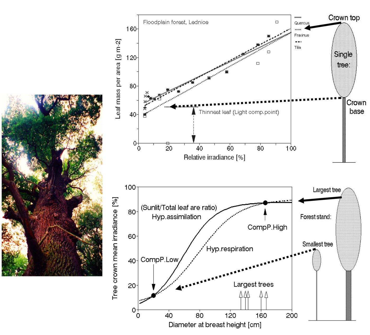
Minimum values of leaf dry mass per area, under which no “thinner” leaves appear, can be interpreted approximately as reflecting individual leaf level light compensation points (Fig. 14, upper panel). Mean relative irradiance of whole tree crowns of individual trees [in % of that above the canopy] can be derived from the whole tree Sunlit/Total leaf area ratio (in % of that above stand - eqn. 4):
Irel-crown can be easily converted to absolute values (Icrown) when the actual values of irradiation measured above the canopy are known. Hypothetically speaking, the Irel-crown curve can be taken as approximately corresponding to photosynthesis at the whole tree level. In analogy with individual leaves, the smallest (and also most shaded) tree of the stand, still may have a rather large diameter (e.g., in the given stand: DBH = 24 cm) and leafed crown, but does not grow (stem growth measured by dendrometer is zero), although it is still alive in the year of the study. This tree approximately represents the situation in which photosynthesis barely supplies enough assimilate for respiration. When respiration becomes greater than photosynthesis, the tree rapidly declines. By analogy to the above-mentioned single leaf light compensation point, we can approximately characterize the whole tree crown in this way as reaching an integrated whole crown light compensation point (Comp. Point low). If this value is calculated for all trees of different sizes within the particular stand, a sigmoid curve is obtained (Fig. 14, left and lower panel). The “assimilation rate” below the compensation point must be lower than the “respiration rate” and vice versa because both curves intersect there. The smallest tree represents the point at which the respiration curve intersects the assimilation curve and was taken as that one reaching whole crown level light compensation point. In larger trees, assimilation exceeds respiration, but no tree of the main canopy can survive below this point. Let us now look at the largest tree. Because the slopes of both curves are slightly shifted, the curves should have an additional intersection point in the region representing the largest tree. Such a tree has a large and relatively very well-irradiated open leaf area, but it has also big amount of respiring tissues (leaves, cambium, phloem, pith rays, fine roots, etc.) and because it is also very well wind exposed, it may in addition loose important parts of foliage when large branches are broken due to heavy winds during storms, etc. Its actual assimilation is than not sufficient to supply their demands (e.g., breaking a single large branch might be critical). Therefore it is supposed, that here its crown can reach another compensation point (Com. Point high). This is assumed as the hypothetical energetic limit of tree growth. Calculated in this way, the maximum energetically limited tree size is within the range of that of the five largest trees growing in the close-to-natural forests in the region ([40]), which suggests, that this hypothesis approaches reality (see Fig. 14, lower panel). Because the precise measurement of such variables is very difficult, we should take this hypothetical calculation only as an example of the eventual possibility of further application of measured and statistically derived data and as a stimulus for the appearance of new viewpoints.
Hydraulic and nutritional limits of tree growth
Ryan et al. ([201]) proposed the hydraulic limitation hypothesis as a mechanism to explain universal patterns in tree height as well as tree and stand biomass growth: growth in tree height slows down as trees grow taller, maximum height is lower for trees of the same species on resource-poor sites, and annual wood production declines after canopy closure for even-aged forests. These authors determined that leaf-specific hydraulic conductance is often but not always lower in taller trees. They confirmed our finding that leaf mass per area is greater in taller trees (indicating better illumination of their crowns). They also concluded that hydraulic limitation of gas exchange with increasing tree size is common but not universal and that further research should consider the more fundamental question of whether tree biomass growth is limited by carbon availability. When one takes into account that carbon availability is also dependent on assimilation/respiration balance, this statement confirms the energetical hypothesis. There is a comprehensive amount of information on the importance of nutrition for plant growth and impacts of its limits ([137], [209], [134], [203], [110]), which represent an excellent basis for further applications of this scientific field. However, ways of development and/or improvement of fast working methods capable to measure and evaluate particular situations at the tree and stand levels are still opened.
Stems (large tree trunks) [6]
Skeleton distribution
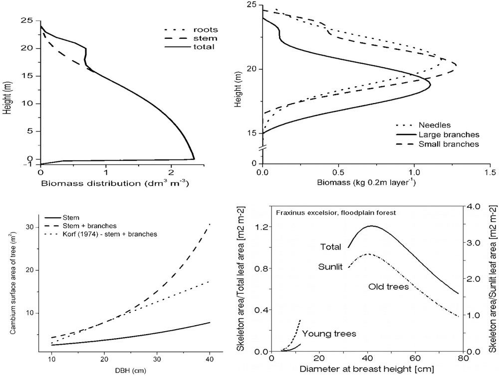
Traditional biometric studies especially considering stem volume or weight represented the basis of forest inventories for centuries. Such results included in all classical dendrometrical textbooks (e.g., [204], [224], [149], [92], [180], [7], [118], [184]). Tables or software are important from the viewpoint of timber production or carbon storage clearly even now. However, in addition to traditional forest inventory data, also other parameters of tree skeleton are important. This means smaller parts of trees (e.g., branches from thicker ones to shoots), but especially their physical parameters as surface area and water content. Such studies are not so frequent (e.g., [127], [95], [231]), but represent important results and non-traditional information (e.g., cambium area index, CAI, or CAI/LAI, etc. - Fig. 15), which indicates how large leaf area supports cambium area unit. These and other combinations of similar parameters are eventually applicable in production studies.
Fig. 15 - Examples of skeleton distribution (in biomass, volume, surface area, water content, etc.) in coniferous (primary data area shown in the first three panels for Pinus sylvestris - [231]) and broadleaf species (relationship of two paramenetrs on the lower right panel are shown for Fraxinus excelsior - [95]); e.g., skeleton surface area in ash (close to cambium area) can be characterized by the allometric relationship: y = {320 exp[-13 exp(-0.064 DBH)]}. Such equations as well as similar others can be applied in many different ways.
Pulsing acoustic tomography
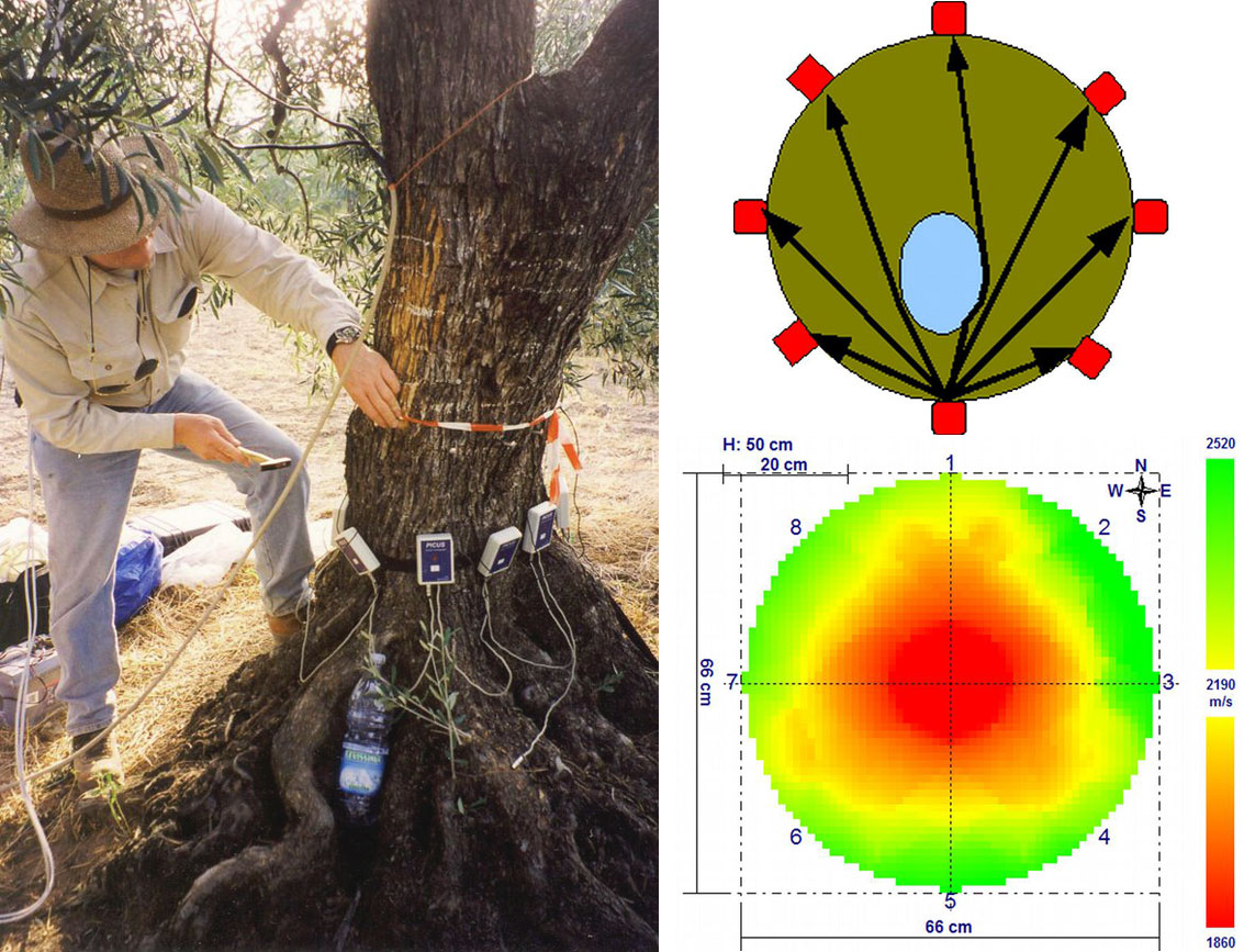
Estimation of the functional and mechanical state of the trunk base and large skeleton roots, particularly in old and large trees, is a very important issue, because falling limbs (e.g., in cities, alleys and parks) are dangerous to people. The static stability of trees is strongly dependent on the condition of the trunk cross-section; here, rot caused by various species of wood-decomposing fungi usually plays the most important role. Pulsing acoustic tomography ([195], [196]) is much more useful for this purpose than xylem core sampling and other destructive methods (Fig. 16, left panel). Pulsing acoustic tomography measures the speed of sound released (and sensed) at a series of points (microphones) situated around tree trunks (Fig. 16, right upper panel). A color image of the whole trunk cross-section obtained through special software can be calibrated in terms of healthy and diseased wood, and the level of decomposition of the wood can be ascertained. In Fig. 16 (right lower panel), which shows an example of a 300-year-old oak tree approximately 180 cm in diameter at breast height, layers of healthy wood (green color) are visible at the east trunk side, and partially (yellow) and completely rotten (red color) areas are also visible. In fact, it is difficult to precisely understand the situation from this data because wood structure also plays an important role, and the color of the images must be interpreted differently in different species. This is an example of an area in which there is room for further methodological improvement.
Fig. 16 - Measurements of structural anomalies (e.g., holes) and health state (rotten area) in tree trunks by the acoustic scanning: field procedure (left panel). Scheme of sound tracks coming from one point to other points (microphones) - the same procedure is applied on all points, and visualizes inner anomalies (right upper panel). Example of a large tree trunk with visualized sound speed (right lower panel - see the scale on the right), indicating healthy (green) and rotten (red) parts of the trunk.
Georadar (ground-penetrating radar) for stems
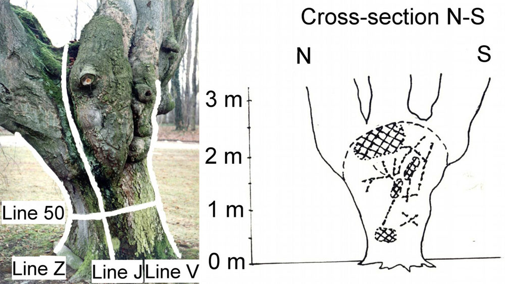
Although georadar is primarily used for root or soil studies (see the next chapter), it can also be applied to the analysis of large tree trunks. Georadar can detect the state of health of stems and reveal the presence of rotten parts and cracks, among other conditions. In this technique, antennas are moved along and around tree trunks so that a 3D image (sometimes a 2D image is sufficient) is obtained. This is shown at scheme of field measurements (Fig. 17, left panel) and at the resulting simplified 2D image after data evaluation (Fig. 17, right panel) according to Hruška ([96]). This technology is very suitable for arboristic purposes and has the advantage that it does not require official paperwork, unlike situations in which radioactive material is applied for similar purposes; the results that georadar provides are sufficiently accurate for practical use.
Fig. 17 - The georadar image of old tree trunk. Positions of georadar lines where antennas were moved are marked on the tree trunk by thick white lines. Different damages within tree trunk are marked at the scheme: wet and porous parts (cross-hatched areas - left panel), cracks and discontinuities (= dashed lines -> right panel: [96]).
Electrical resistance or conductivity
Fig. 18 - Measurements of structural anomalies based on electric scanning (Gottingen University Team 2004). Cross-section of beech tree trunk severely damaged by rot (upper panel). Rotten parts of tree trunk visible on the image (modified from [88] - middle panel). Trunk base admittance in milli-Siemens measured by the long column method using alternative current in a series of Norway spruce trees growing at the peat land. Most of them are close to generalizing line, those markedly above it indicated partial trunk wet rot; those below have several dry branches at the top (lower panel).
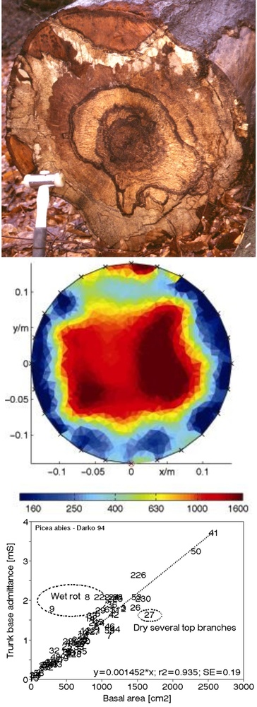
Multielectrode resistivity imaging of rooted soils ([3], [4], [5]) or stems ([90], [91], [88]) is a rapidly developing method that is very useful in field studies. This method can be used to visualize the distribution of soil volumes with different root densities or root biomasses and to distinguish healthy and rotten parts of stems. It provides results similar to those obtained from pulsing acoustic tomography for rooted soils and stems but with greater detail (approximately 1-cm resolution) when larger series of electrodes are used ([90], [91], [88], [89]). Holes in stems, their rotten parts and sapwood can be distinguished (Fig. 18, upper and middle panels). Only 4 electrodes (2 current C electrodes, C1 higher (4-6 m) in the stems and C2 in the soil and 2 potential electrodes (P1, P2) at a small constant distance (Lel.stem = 0.2 to 0.3 m in the lower part of the stems) are needed to quickly estimate the whole tree stem (of the diameter, Dstem) electrical conductance (or stem resistivity, ρstem) of many trees when anomalous sample trees in stands should be avoided. Resistivity ([Ω m]) is than calculated as (eqn. 5):
This technique, however, does not permit detailed analysis of stem structure (Fig. 18, lower panel).
Root system [7]
Classical excavation technologies
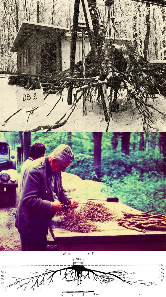
Root system analysis was a very difficult task when only manual excavating methods were available ([106], [104], [119], [120], [235], [109], [176], [113], [114], [115]). Only skeleton roots could be opened this way; the morphology and anatomy of these roots has been analyzed perfectly by several authors, but root systems are difficult to quantify, even when sophisticated methods are applied ([176], [222]). Probably the best-illustrated book on both skeleton and fine roots including their microscopy analysis was done by Kutschera & Lichtenegger ([131]), where the authors applied thin metal needles for manual root excavation. Example of large tree excavation using large instruments (crane, big reservoirs with calibrated scale) and a lot of manual work is shown in oak trees from a floodplain forest, where the published data ([235]) represent accurate drawings (based on precise photo images) and corresponding dry weight and volume tables (Fig. 19). It is clear, that such studies are very cumbersome, demanding in manual power and time consuming. The obtained general views of morphological parameters are valuable, also description of mass and volume of root skeleton. However quantification of gentle root structures as fine roots by these methods is very difficult. Therefore their application for forest level studies requiring wider application in burdensome terrain conditions, or repetition across many sites and species is very limited.
Fig. 19 - Measurements of (aboveground and belowground) skeleton distribution in large trees using classical destructive methods (floodplain forest near Lednice, southern Moravia - according to [235]). Volumetric measurements of whole stumps using a small crane and a large water-filled metal reservoirs with a calibrated scale (upper panel - photo: Vyskot, 1971). Manual work of many anonymous technicians when sorting roots according their diameters (middle panel). Side view of root system redrawn from precise photo images (lower panel), corresponding to the quantitative data on dry weight and volume given in tables.
Supersonic air stream
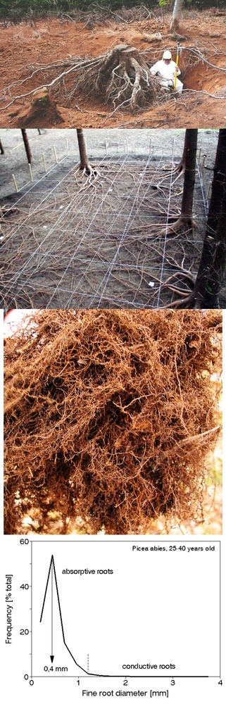
Obtaining an accurate description of the usually invisible parts of trees’ root systems is of great importance. Cumbersome and laborious manual root excavation has today been replaced by the supersonic air stream method (the “air spade”), in which a very thin stream of air moving from a nozzle attached to a strong compressor at a speed of Mach 2 is applied ([197], [173]). Smooth objects (e.g., stones, roots, bare feet) are unaffected by the air stream; however, when the air stream reaches a small pore, the air is compressed within the pore, and the pore explodes. Soil is dispersed by micro-explosions in a cloud of dust this way and moved away, while roots remain almost untouched. However, they may be slightly damage at the surface by fast-moving sand grains and some fine roots may be destroyed (Fig. 20, top panel - [69]). When soils become hard during drought, fine roots can be damaged significantly by this technique because they are held tightly by soil and the soil itself is only partially dispersed; that is, large pieces of soil (clods) hold fine roots tightly. When air pressure is applied, the clods are then moved away as a whole, carrying fine roots with them. However, when roots are wet during excavation, most roots will survive, and the tree continues to grow when the roots are again covered by soil. Root opening can be accomplished quickly when only a shallow soil layer is removed (e.g., 10 m2 per hour to 0.5 m depth - Fig. 20, second panel). Fine roots can also be opened, provided the work is done very gently under conditions in which the soil is sufficiently wet and soft (e.g., in pieces of decomposed wood). We can see it for example in spruce (Fig. 20, third panel) where their absorptive part reached in average its diameter modus of 0.4 mm (max up to 1.2 mm - Fig. 20, fourth panel), mean length of almost 3 mm and density over 300 000 tips per m2 of stand area ([70]). In deeper layers (e.g., at 2.5 m), this method is much more time consuming because the root network usually makes it difficult to remove larger soil particles and stones from the hole and it is sometimes necessary to remove stones manually. Roots can be photographed and the images elaborated by the image analyzer method, if necessary. The supersonic airflow method is also suitable for some construction work, e.g., when it is necessary to lay cables or pipes in soils while avoiding the type of root damage that would occur when using picks, excavators or bulldozers.
Fig. 20 - Visualization of the whole tree root systems by the supersonic air stream (the “air spade”). Root system of a Douglas-fir (Pseudotsuga menziesii) tree opened down to the depth of almost 2 m (top panel). Notice the nozzle hold by the operator with the hose going to strong compressor situated near-by. Root systems in a group of Norway spruce (Picea abies) sample trees up to a depth of about 40 cm, and down to 75 cm in places where sinker roots occurred (second panel). Detail of a bunch of Norway spruce fine roots (down to diametersbelow 0.4 mm), found in extremely soft soil within the almost decomposed stump, which occurred about 10 cm below the ground surface (third panel). Diameter of spruce fine roots characterized by detailed biometric (and microscopic or their function characterizing) data, well distinguishing their non-suberized (absorptive) and suberized (mostly long-distance conducting) parts (fourth panel - [70]). Rough assessment of diameter categories only without similar evidence is not sufficient for fine root quantification, modeling, etc.
Pulsing acoustic tomography
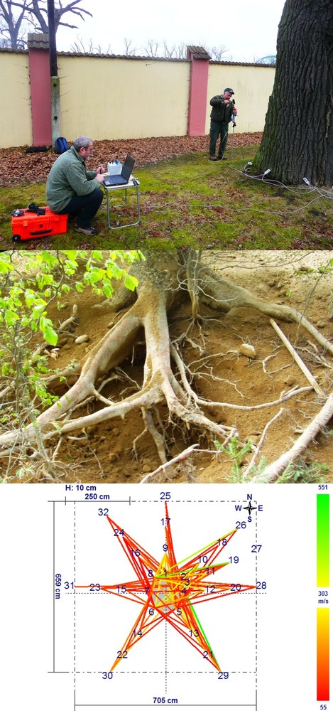
Pulsing acoustic tomography can be also used to measure the distribution and functional state of large skeleton roots ([207]). A large hammer generates the sound, which is sensed by a series (e.g., 12) of microphones installed at the base of the tree (Fig. 21 - upper panel). The sound pulse moves through 2 different media, soil and roots, in the form of a mechanical wave that is described by the Lamee’s equation ([133]). When the sound wave touches the root, longitudinal and tangential waves are generated, particularly at lower frequencies; these waves then move to the microphones (Fig. 21 - middle panel). Evaluation of this process is more demanding because of the difficulty of calibrating the state of the root. By contrast, the root distribution around the tree can be estimated rather easily. In the example shown in Fig. 21 (lower panel), it is clear that the roots are rotten on the same side as the trunk itself. On this basis, the tree can be classified as clearly unstable and risky; however, its condition is not visible because the rotten part of the trunk is still covered with bark. To prevent any casualties, a similar analysis should be applied in a timely way everywhere old trees are situated. The output data can be analyzed in more detail by special software that provides a mechanical model of the trunk, which can even give the direction of possible trunk destruction and potential falling of the tree.
Fig. 21 - Acoustic image (pulsed acoustic tomography) of large skeleton roots around tree. Photo characterizes typical fieldwork, when one operator is periodically hitting an anvil that is moved around trees and the second person checks the data on a computer screen (upper panel). An example of the root system partially opened by the air-spade (middle panel) and the image of its individual branches with visualized healthy and rotten parts (lower panel). For image interpretation see the scale (sound speed in m s-1): green color (indicated high sound velocity) means healthy tissues, red color (indicated low sound velocity) means rotten parts of roots and yellow is the transition zone.
Georadar (ground-penetrating radar) for roots
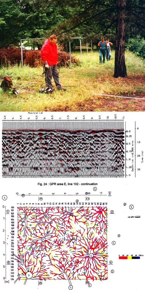
Georadar was introduced to root studies by the geophysicist ([97]) and has frequently been used for root analysis since its introduction ([241], [60], [24], [25], [217], [6], [12], [76], [183], [88], [89], and many others). This method can “see” small objects such as “finger-sized” roots, which can be visualized to a depth of approximately 2 to 3 m, and thinner roots to a depth of approximately 1 m using different frequencies and antennas. The antennas are usually moved manually along lines (e.g., tapes) across the measured sites (Fig. 22, upper panel). The system detects point reflections from contrasting materials. The primary radar images usually include many reflections from roots, stones and other particles, yielding thousands of reflections for each sample tree. In this way, 2D “slices” of soil and other materials are obtained (Fig. 22, middle panel), and 3D images are reconstructed from a series of such slices by special software. This method can “see” large objects (stones, old house walls, etc.) to a depth of 30 to 60 m; and thinner “pencil size” objects to a depth of approximately 1 m using different frequencies and antennas (Fig. 22, lower panel). When working in cities, a particularly useful attribute of georadar is, that it can “see” roots through concrete walls (e.g., roads, pavements, bottoms of concrete pools). The work is relatively easy in homogeneous soils, but problems occur in soils with large fractions of stones or gravel; these are sometimes difficult to distinguish from roots, and this can cause large errors. Horizontal roots can be visualized better than vertical roots, which run in parallel with the radar beams. The computer-generated images can be evaluated by the image-analyzer method. Georadar is also suitable for the analysis of subsoil or soil water distribution ([135], [94]) at the level of entire forest stands. Radar application is more difficult in electrically highly conductive soils containing clay, which limits the resolution and detection depth, and in stony or gravel soils, where many false reflections interfere with those from roots ([98]). However, the method can also be applied to the analysis of subsoil distribution (e.g., detection of deeply situated rocks, old river beds, etc. and/or selection of representative sites for soil sampling), where its resolution is sufficiently high to characterize, e.g., 1 ha using a similar number of measuring points as for single trees (Andreas Kathage, cited in [88]).
Fig. 22 - Ground penetrating radar (georadar) system. Field procedure of measurements, Antennas are moved along the tape in regular intervals and the images are taken in each step (upper panel). Recorded image - reflexes from different objects in soil characterizing one cross-section of the measured site (its “slide”), which is the material for software analysis (middle panel). Image of the root system of a medium age (Picea abies) trees to the depth of 80 cm (depth marked by colors shown at the scale on the left; modified according to [98] - lower panel).
Tree-water relations
General problems of field-measured variables
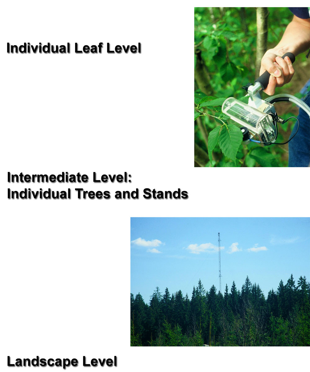
In general, plant-water relations are closely connected with the flow of energy in ecosystems. Water is the most frequent limiting factor for growth, and it provides the necessary background for other physiological processes. Current technology makes it possible to measure quantitative parameters of water relations, carbon flow, growth and structure at the level of plant organs, whole trees and entire stands, as well as their combinations at the level of watersheds or larger forest areas. Each level of such studies with its instrumentation has its most suitable applications and also limits. For example, individual leaf of root studies based on gasometrical methods allows very detailed and precise laboratory approach or analysis of the small parts of plants (e.g., in agriculture), or easily accessible parts of larger plants (Fig. 23, upper panel), but there are problems with up- scaling data for higher levels of biological organization. Micrometeorological methods (dependent on tall towers) provide very valuable large-scale data, but they are dependent on wind directions and have problems in distinguishing contrasting behavior of measured objects, e.g., include information about forests (but not individual species), lakes and villages if in the same direction (Fig. 23, lower panel).
Fig. 23 - Eco-physiological studies (here focused on gasometry) in trees at different scales: Small- individual organ scale, e.g., leaf level. Manual work on a tower is shown in the picture from Harvard forest (upper panel). The intermediate scale is illustrated in following figures. Large scale - landscape level (hydrological and micrometeorological methods, e.g., eddy covariance) as applied in flat area e.g., by Uppsala University in southern Sweden, where a 100 m tall tower was constructed. (lower panel).
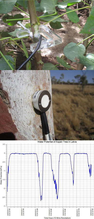
Mobile, field-applicable instrumentation based on whole tree and stand level approaches is independent of built stationary objects (greenhouses, towers, scaffoldings, etc.) and can easily characterize individual species, trees of different size and social position, groups of healthy and damaged trees. Radio-equipped dataloggers allow automatic recording and data reading on long distances. A present (but gradually diminishing) disadvantage is that they cannot measure all-important physiological processes yet. But there are many measurable variables characterizing tree water relations. For example, Schlolander’s bomb has been very popular for measurements of leaf or shoot water potentials. An automatically working stem psychrometer (Dixon’s system) appeared on the market most recently and it is suitable for both: small (Fig. 24 upper panel) or larger stems (Fig. 24 middle panel) of non-resinous tree species. This provides a possibility to get continuous (or very short periodical) records for the first time (Fig. 24 lower panel). However, the most useful and popular is sap flow (xylem water flow in stems or branches), because of long-term experience with its measurements, series of different available methods, automatic recording and valuable integrated information, which this variable provides.
Fig. 24 - Stem psychrometer according to Dixon. Installment on small trees or branches (upper panel) and on large tree stems (middle panel). In both cases the sensor must be sealed to the stem in a waterproof manned and well insulated. The example of diurnal records of sap flow is shown on the lower panel (all according to ICT International materials).
Sap flow in trees [8]
Measurements of the sap flow rate in trees
Sap flow or transpiration dynamics was one of the first phenomena to be studied in tree-fieldwork in the late twenties ([99], [100]), if one does not consider the indirect methods applied by a genial scientist Stephan Hales ([93]) in much earlier plant physiology studies. Studies of sap flow offer the great advantage that when sensors are installed on tree trunks or stems, they integrate the behavior of the entire crown and/or whole tree root system, and these parts as well as stems can be evaluated separately. We began developing instrumentation for this purpose in the late 1960s, resulting in the trunk heat balance (THB) method (Fig. 25, upper panel, see also Fig. 26, upper panel). This robust method is based on the measurement of power (an electric current which is separated from ground and passed through xylem tissues) and temperature differences in sapwood. It measures the size-defined and largest stem sections of all the section-based sensors (40-80 mm) and integrates flow over sapwood depth by two thermocouples in different sapwood depth, but also by the “self adjusting” current, which does not pass through dry heartwood (if electrodes are installed deeper), but passed through sapwood if electrodes are installed shallower (because of their distance). THB gives the total sap flow rate across the sapwood area of trees ([49], [50], [63], [132], [33], [80], [221]). At least two measuring points from the opposite sides of the stem should be used. The most recent version of this method can measure even zero and bilateral flows (usually acropetal, but also stress-characterizing basipetal flows) when applying horizontal position of thermocouples ([226]). The heat ratio (HRM) is probably the best pul- sing method based on the ratio of temperature differences in a logarithmic form, measured up-flow and down-flow at the period before and after the pulse ([22]). Each sensor has two thermometers in each of two vertically applied needles plus a needle heater between them in order to integrate partially the radial pattern of flow. It works in a pulsing regime, considering the ratio of temperature values before and after the heating pulse. The system can measure zero and reverse flows in small and large trees, if their sapwood is not too deep (Fig. 25, middle panel). The heat field deformation (HFD) method is based on the ratio of heat flow (through temperature differences) in the axial and tangential directions around a linear heater (Fig. 25, lower panel, see also Fig. 26, lower panel) and was developed in the mid-1990s ([163], [165], [170], [162], [63]). The HFD method permits measurement of flow at many points along the stem radius by multipoint sensors ([30]) and therefore provides information on the radial pattern of sap flow. It can also measure bilateral flows. The method is based on measurement the asymmetry of the heat field around the heater (low asymmetry = low flow, high asymmetry = high flow). THB and HFD multipoint sensors are equipped with all electronics and a series of 6 to 8 thermometers in each needle, which are of different lengths and therefore can cover sapwood of different depths, ranging usually between 2 to 12 cm (max. 25 cm with 10 thermometers inside).
Fig. 25 - The trunk heat balance (THB) method (upper panel). Temperature difference, dT is measured in the vertical (axial) direction by a series of thermocouples (which, in the displayed version, are shown situated at the center of electrodes, therefore partially integrating the temperature of the electrodes). The most recent variant of the sensor with constant gradients and constant dT (1-2 °C) heating electronics is available from EMS Brno. Variant with horizontally situated reference thermocouples measures also zero and reverse flows. The HRM method (middle panel) applies the most sophisticated pulsing system available. Two needles with pairs of thermometers are situated above and below the needle heater. The HFD method (lower panel) is based on linear radial heating (by a resistance wire inserted in the central needle at the picture). Two needles are inserted up and down the heater (at distance 15 mm) and on one or both sides of the heater (5 mm). Each needle contains one or a series of thermocouples (in the multi-point sensor), measuring temperature at different depths. Therefore the sensor also measures zero and reverse flow and flow density in different depths.
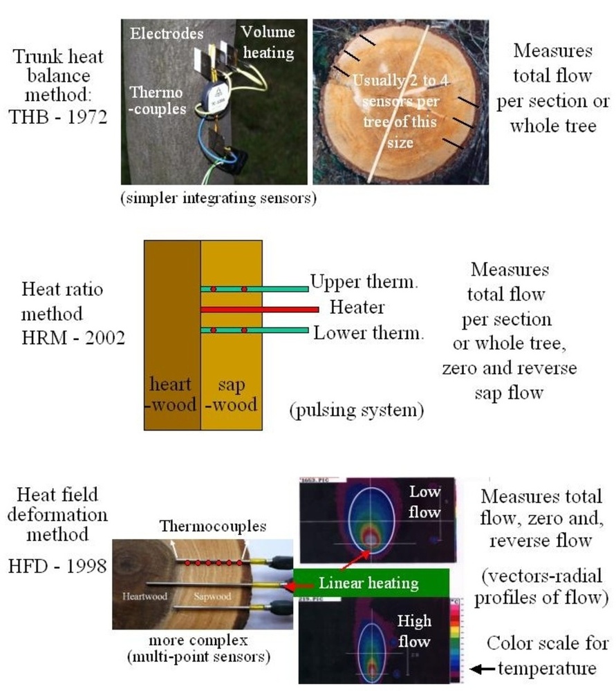
Fig. 26 - Trunk heat balance (THB) sap flow sensor with dT const system (EMS Brno, Czech Republic): Sap flow module EMS 51.1. (size 160 x 80 x 50 mm, upper panel) includes a set of single point temperature sensors in hypodermic needles, and a set of 40 to 80 mm long electrodes. They are supplying heating power to the sapwood (with an insulated part for phloem layer) and providing flow data, which integrate the whole sapwood depth. Electronic circuit controls power on the basis of evaluating signals from thermometers and another electronic circuit for measurements of electric conductivity of xylem between electrodes. It works with dT = 1 to 4 K, Ub = 12 V, output 0.8 mW K-1 mV-1. Optical outer signaling system is used to control power, error, fuse and polarity. Datalogger can be installed inside on request. Heat field deformation (HFD) multipoint sap flow sensor, (ICT International, Armidale, Australia, size: 270 x 80 x 30 cm - lower panel) consists from the needle heater (red, 115 mm long) and a series of three needles, each containing eight thermometers (black, 95 mm long). The constant power (0.1 W cm-1) heats the needle uniformly along its whole length. The sensor contains a battery, small datalogger and a radio set allowing reading and downloading the data from a long distance.
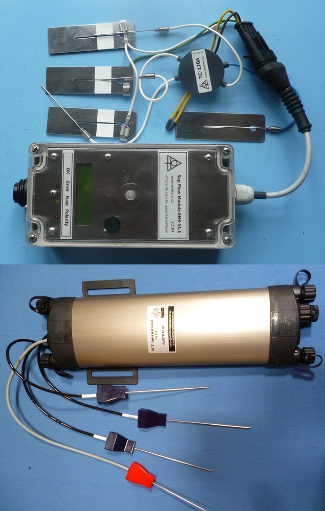
Integration of sap flow across stems
As mentioned above, the measurement of sap flow has the great advantage that, when sensors are installed on tree stems or large trunks without branches (e.g., from approximately breast height up to the first living branch), they integrate the behavior of the whole tree crown and/or the whole tree root system. If a separate evaluation of crown or root branches is needed, the sensors should be installed closer to the region of interest. However, when attempting to quantify flow values for the whole tree, it is necessary to consider their spatial variation by using a series of measurement points over the entire depth of the sapwood and entire stem girth. In small young trees, sapwood can cover the whole cross-section area, but in large old trees, it is limited to the outermost layers of sapwood. It can be wider (deeper) in conifers or diffuse porous species (Fig. 27, top panel) and narrower in ring-porous species (Fig. 27, second panel). Of course, it is variable according to local growing conditions. Problems arising from variations in the spatial flow can be overcome by the application of technically integrated sap flow sensors in THB systems or by measuring radial patterns of flow along the stem radius in HFD systems. In both cases, the circumferential flow variation should also be considered because flow values along the xylem radius, as well as along its circumference, can differ by as much as an order of magnitude (Fig. 27, third panel). Estimation of sap wood biometrical characteristics, i.e., its depth below cambium expressed in absolute or relative values of stem radius (Fig. 27, fourth panel) is recommendable especially when starting the work with new species, etc. When using flow sensors based on outer stem heating and dT sensing in small branches, it is not necessary to consider such variation because these devices provide total sap flow per branch automatically. However, additional measurement points should be installed around stems; in the THB system, at least 2 wider measured sections from opposite stem sides (e.g., up to 8 in very large trees) should be used, while in the HFD system, at least 4 narrower measured sections are required (in both systems, more sections should be used in large trees). The measured sap flow per section is converted to flow per tree according to the ratio of section width to xylem circumference (in THB) or to the total sapwood depth (in HFD), or area when summarized (see Fig. 27, fourth panel). More details are provided in Cermák & Kucera ([32]), Cermák et al. ([63]), Nadezhdina et al. ([170]) and Nadezhdina et al. ([171]).
Fig. 27 - Rather wide sapwood (more precisely wetwood) visible on the stem of large spruce tree (green color is caused by algae - upper panel). Narrow sapwood in ring-porous pedunculate oak (second panel). Spatial variation of sap flow density in radial and circumferential directions across the Scots pine tree trunk, measured by a series of 4 multi-point sap flow sensors (altogether in 48 measuring points). Radial pattern of measured sap flow density and derived flow per individual annuli in a sample tree, where sap flow in the outer and inner sapwood layers was distinguished. Scale is in g cm-2 h-1 (third panel). Relationship of relative sapwood depth (taking xylem radius as independent variable) in a series of broadleaf and coniferous tree species (Quercus cerris, Q. pubescens, Populus interamericana, Picea abies, Pinus sylvestris - fourth panel). Most trees were growing in medium deep soils. A group of deviating pine trees was growing on very deep and dry sandy soil. Summarized data from several studies ([67], [221], [167]).
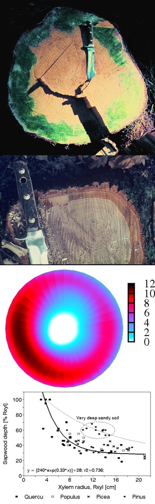
Variants of all three methods have been applied to small trees, branches and roots. For example, the Baby THB method has been using the external contact heating and sensing ([51], [136] - Fig. 28, top panel). HFD uses shorter or asymmetrical sensors for this purpose ([178] - Fig. 28, second panel). Heat ratio method (HRM - [22]) applies sensors, which can be applied for large as well as for small stems or branches (Fig. 28, third panel). Palm stems or large leaves can be best measured with the long HFD multipoint sensors, which can easily measure flow in the outer as well as in deep layers of conducting systems (Fig. 28, fourth panel). All these types of measuring instrumentation are commercially available. Trunk heat balance systems from EMS Brno, Czech Republic, and heat ratio plus heat field deformation systems from ICT International, Armidale, Australia.
Fig. 28 - Sap flow meter based on the THB method with external contact heating installed on the petiole (5 mm in diameter) of a large leaf of Ailanthus glandulosa (top panel). Sap flow meter based on the HFD method installed on the small (25 mm in diameter) stem of Fagus sylvatica sapling (second panel) and in the branch by the heat ratio method (HRM) (third panel). Thermometers are switched off in that part of needles, which are outside the measured stem. Sap flow measurement by the multipoint HFD sensor in the large leaf of palm (fourth panel), where most flow goes through its center.
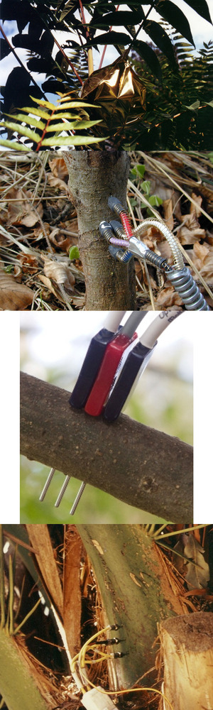
Variation of trees and their parts where sap flows
Examples of forest stands where sap flow meters should be installed include aged Norway spruce plantation, Sumava Mountains, Czechia (Fig. 29, top panel), uneven-age mixed forest stand with large trees and seedlings from natural regeneration near Volga river source, Russia (Fig. 29, middle panel) and a stand with very large Douglas-fir and Hemlock trees, West Coast virgin forest, Wind River Research Plot, USA (Fig. 29, lower panel).
Fig. 29 - Example of different experimental plots with a series of sample trees of different size and social positions: (1) Mature Picea abies plantation in the Šumava mountain forest, Czech Republic (upper panel). (2) Naturally regenerated mixed lowland forest near Pyeno, Russia with coniferous (Picea abies, Pinus sylvestris) and broadleaved woody species (Populus tremula, Betula alba, Sorbus aucuparia). (3) Sample trees of different size and age. Single-point HFD sensors were applied on small trees and multi-point HFD sensors on large trees (middle panel). THB sensors were applied in a mixed forest including species (Pseudotsuga menziessii, Tsuga heterophylla, Acer macrocarpa) and trees of different age in the virgin Wind-River sub-mountain forest in Washington, USA. These trees were much larger than in Pyeno (DBH > 200 cm, height 60 m) and were growing on volcanic soils (lower panel).
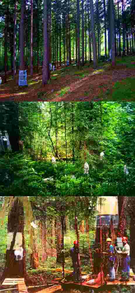
Selection of stand-representing sample trees
Distribution of trees of different diameters can be very variable and species composition in stands should also be considered, because the impact of social position can differ between species (Fig. 30, upper panel). Therefore selection of sample trees truly representing a stand is not always easy when applying classical methods (especially in stands with more variable structure). When measuring any dendrometric variable at the stand level using a series of selected sample trees whose number may be limited for technical reasons (such as numbers of available measuring channels), it is desirable to select sample trees that best represent the particular stand. In practical terms, this also requires a proper use of the eventually applied stand-representing technology so that, e.g., each channel measures a tree representing the same or a very similar part of the stand. In situations in which the importance of tree social position from the standpoint of water consumption is dependent on species, root system and crown density, sample trees should encompass the entire range of tree sizes present.
Fig. 30 - Evaluation of social position of trees according to relative stand-level transpiration in three different species and site conditions - floodplain forest: Quercus robur, upland: Picea abies and lowland: Pinus sylvestris. Each social group represents the mean of the same stocking density per 1 ha (upper panel). Selection of the representative sample tree sizesfor the analyzed stands using the statistical procedure of quantil of total. This procedure simultaneously considers tree size (e.g., basal area, Abas) and stocking density. Each selected sample tree represents the same fraction of selected biometrical parameter of the entire stand. This is best calculated when accumulating data from individual trees, which can be found according their DBH in the field (middle panel), but it is also possible to apply DBH classes with very little increasing error (lower panel). Diameter at breast height of each particular selected sample tree (DBHi) correspond to each particular mean value of Abas-i - see arrows.
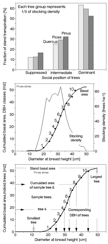
Sample tree selection should simultaneously integrate tree size and tree density in the stand. This can be done by applying a statistical approach called the “quantils of total” ([31], [34]). The quantil of total represents the value of a chosen, most suitable dendrometric variable (e.g., basal area, leaf area, timber volume) that is in the “center of gravity” of an assortment of trees (the entire stand or its part). If a single sample tree should be selected, the method divides the stand total, e.g., a basal area of 52 m2 ha-1, into 2 identical parts and the representative size of sample tree, which can be read from the cumulated curve (e.g., Gompertz) would corresponds to the stand basal area value of 26 m2 ha-1 (a vertical line drawn from this point down indicates the DBH of such sample tree). When (as usual) more sample trees should be selected (e.g., 10 or more in mixed forests), the quantil of total divides the stand into 2 halves for each particular basal area total, which is again identical for each sample tree (Fig. 30, middle panel). The values of each particular total are obtained by calculating a cumulative sigmoid curve of all trees per hectare in increasing order (e.g., these 52 m2 ha-1) and dividing this value by the required number of sample trees. In this case, each particular total is 52/10 = 5.2 m2 ha-1, its half = 2.6, and the derived quantils are 2.6, 7.8, 13.0, …, 49.4. The corresponding DBH of the sample trees is then readable from the corresponding sigmoid curve (Fig. 30, lower panel). The detailed description of the method with more examples and including corresponding tables etc. is available in the specialized methodical paper ([63]).
Up scaling of sap flow to different levels of biological organization [9]
Sap flow data from sample trees to forest stands - forest inventory
When results at the level of forest stands or orchards are required, a series of well-selected individual sample trees (see Fig. 30) must be used, and the data can then be scaled-up to the entire stand area (e.g., 1 ha) or higher levels. This can be done on the basis of forest inventory data, eventually including some more detailed parameters such as the sapwood area. We have measured tree sap flows and relate their daily (or hourly) values to the above-applied biometric data (e.g., DBH, basal area). A sigmoid curve (e.g., Gompetrz) has been usually calculated from individual points representing sample trees, and mean values for each DBH class were derived on this basis. In relatively young trees and uniform stands, only the first part of the curve appears (Fig. 31, top panel). In such stands we are getting results with minimum scaling error, say 5% (Fig. 31, second panel). If the stand is older or for some reason is more limited in its development, the upper end of the curve becomes more flat (Fig. 31, third panel). Larger variation between trees naturally causes higher scaling errors, e.g., 10%. Then, in any case the mean value for each DBH class is multiplied by the number of trees in that class of the given stand, and these values are summarized to obtain data for the whole stand. The resulting value represented stand transpiration on the selected day. Transpiration for all days of the time period has been calculated in the same way, taking into account, e.g., the growing season (see [63] - Fig. 31, fourth panel).
Fig. 31 - The relationship between diameter at breast height and daily totals of sap flow in individual fir sample trees growing in homogeneous, young, well growing stand applied for up scaling of sap flow data measured in for the entire stand (1 ha - upper panel). Daily totals of sap flow can be considered as transpiration, because time shiftsand daily differences between dehydrating and rehydrating flows are very small and play no role. Variation of data and corresponding scaling error were relatively small here (second panel). The form of the generalizing curve and variation of the relationship was larger in an old pine stand with more heterogeneous soil conditions (third panel). In both cases, the data generalized by the curves were up scaled from sample trees to the entire stands. Values from the curves for individual DBH classes were multiplied by numbers of trees in classes (see columns) and all classes were cumulated in order to get transpiration for the entire stand (lower panel). This can be calculated day by day and then summarized over the growing seasons as shown here.
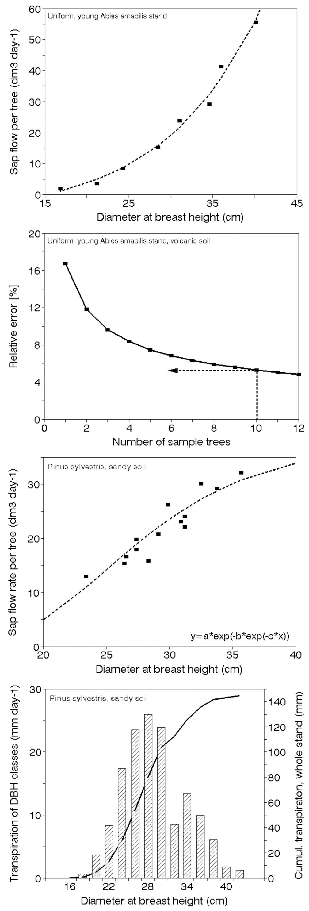
Sap flow data from sample trees to forest stands - remote sensing
Transpiration data can also be scaled-up by a remote sensing approach that has been applied for years (here as modified earlier according to [11] and [31]). An image of the experimental plot with sample trees taken (e.g., at IR-band-7 - Fig. 32, left panel) was analyzed according to image density of the part of the forest, where a series of sample tree is situated (Fig. 32, right upper panel). When the image density is plotted against transpiration of sample trees, it serves as a calibration curve for each studied species (Fig. 32, right lower panel). This analysis requires that images be acquired at the period of time when sap flow Qw is equal to transpiration EQ (i.e., shortly after noon); at this time, we can neglect the time shift between the 2 flows (either when EQ > Qw in the morning or vice versa in the afternoon hours). Comparison of remote sensing data with transpiration measured during other daytime hours requires time shift corrections.
Fig. 32 - Up scaling transpiration from individual sample trees to stands by remote sensing, using image IR_band.7 (left panel), scheme of evaluating the image density (right upper panel) and calculated relationship between IR image density and transpiration Sessile oak and Norway spruce (right lower panel).
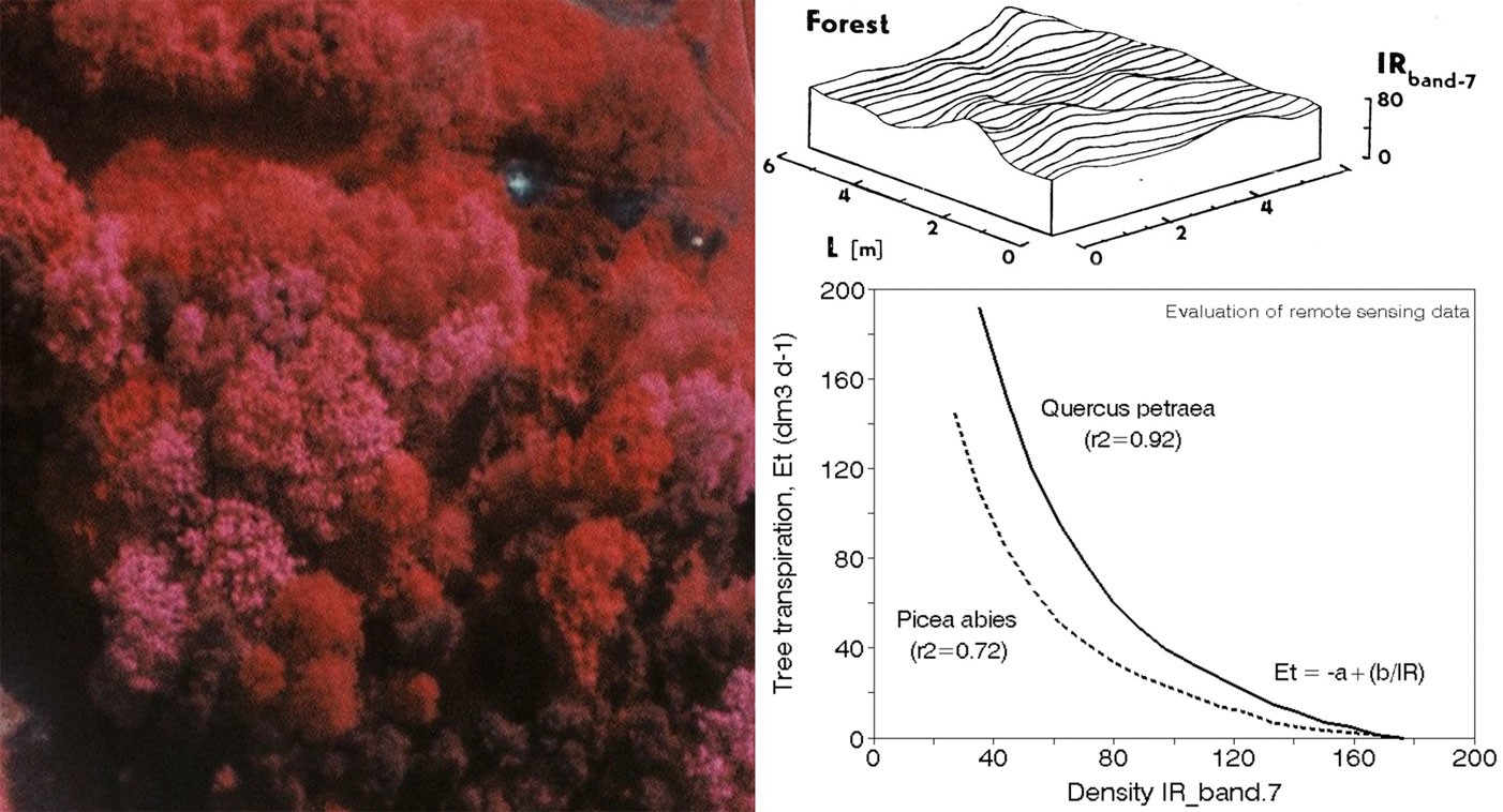
Sap flow data from experimental stands to the landscape level
More variable stands usually occur when larger areas of the landscape, such as forest enterprises or watersheds, are considered. In such cases, it is necessary to select a series of experimental stands encompassing the entire area. These stands can be selected on the basis of forest classification systems (forest typology - see the first chapter), hydrological typology or any other system capable of distinguishing relevant properties of different sites (see Fig. 5). Transpiration representing the entire considered area can be calculated in a similar manner as when scaling-up trees to stands; the typological data can also be used for the eventual constructions of more complex models for the same purpose ([178], [179]). Application of remote sensing technology is especially advantageous here ([73]). In both cases, the landscape representative stands are specified on the corresponding maps and then identified in the field (Fig. 33, upper three panels). Further procedure with a series of stands goes as described above with a single stand. Data obtained in a stand representing a certain forest type is then multiplied by corresponding area of that forest type in the study area.
Fig. 33 - Scheme of the upscaling procedure from a series of well-selected representative stands to the landscape level (e.g., watersheds or forest enterprises). This general map gives the geographical orientation, where the selected stands are situated (upper panel). The detailed map (forestry or geobiocenological map, etc.) helps to select and specify individual forest stands (individual experimental plots marked by squares - middle left panel), which will be found in real terrain (here a remote sensing image is shown - middle right panel) where measurements will be done. An example of modeled data and those measured via sap flow in mixed forests of northern Russia is included. Two models have been applied: for evapotranspiration and transpiration itself. The seasonal course of sap flow and modeled data (lower left panel) and relationships of sap flow (independent variable) to both models (lower right panel) are also shown.
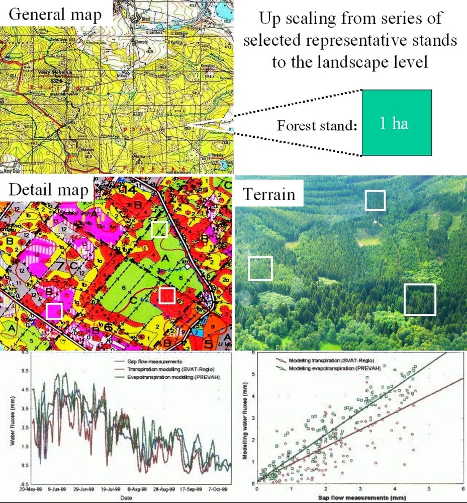
It was found suitable to combine data calculated on the basis of several (here shown two) hydrological models with pixel size (here 4 ha) corresponding to the whole area studied (e.g., 350 000 ha at the Volga river source) and verify them by comparing to sap flow data measured in selected pixels. The evaluation indicated, that results of both models slightly differ from those obtained by sap flow measurements, which was visible on the seasonal record of all variables, but even better when relating modeled data to sap flow (Fig. 33, lower panels). Individual deviations could be specified and results corrected accordingly ([178], [179]).
Sap flow, water storage and stem growth dynamics [10]
Diurnal and seasonal sap flow dynamics
Diurnally measured data obtained by the methods described above are usually recorded in 5-, 10-, 20- and 30-minute intervals. Each firm producing instruments for sap flow measurements also provide corresponding special software, allowing fast field control and evaluation of primary data. Evaluation of total sap flow data measured by the THB method is easier, because the sensors are more simple, although giving total values of sap flow per section; evaluation of data obtained by multipoint sensor of the HFD method is more complicated, but both methods use specific software for this purpose - see an example (Fig. 34, upper panel). Both methods are very sensitive to changes in environmental conditions e.g., during sunny, cloudy and rainy days (Fig. 34, middle panel). Quantitative differences between the diurnal courses of sap flow in pedunculate oak trees of different sizes and under varying weather conditions (fine, cloudy and rainy weather) are also visible in the figure. More details on sap flow in different sapwood depths can be seen on the diurnal records of the HFD sensor. Seasonal course of sap flow (or transpiration EQ, if daily totals are taken into account) are usually compared to the same course of potential evapotranspiration, PET. Ratio of these two parameters (EQ/PET in m2 per tree or in % per stand) is similar to the conductance of the system (which is described in another chapter). It is almost constant under sufficient and stable soil moisture (Fig. 34, lower panel), but decreases significantly under drought or disturbance by any other factor (e.g., hypoxia, mechanical, fungi or insect damage, etc. If introducing sap flow for individual trees, we would get the effective projected crown area, Aeff , in m2 per tree.
Fig. 34 - Diurnal courses of sap flow rate measured in different sapwood depths by the multipoint sensor (HFD method) during data evaluation by the Sap Flow Tool (ICT International - upper panel - modified from Proc. of 9th Sap Flow Workshop, Ghent 2013). Diurnal courses of sap flow rate (THB method) in a series of individual pedunculate oak sample trees of different size during fine, cloudy and rainy weather, illustrating possible range of dynamics (measured by any of the mentioned methods) occurring during this period of time (middle panel). Seasonal course of sap flow rate or transpiration (EQ, daily totals) in the entire stand (full squares) of floodplain forest with non-limiting soil water supply and potential evapotranspiration (PET, empty squares - lower panel). Full thin line represents calculated relative transpiration of the stand (EQ/PET in %) and dashed line characterizes its seasonal trend under given stable environmental conditions. It would fall down after depletion of soil water (if introducing sap flow for individual trees, we would get the effective projected crown area, Aeff , in m2 per tree).
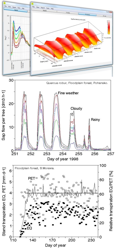
Dendrometers and stem growth
Manual band dendrometers are well known, extremely simple, inexpensive and easy-to-use instruments. Band dendrometers can provide valuable data on stem circumference if an accuracy of 0.1 mm and periodical manual reading (taken, for example, over 1- to 2-week intervals) is sufficient time resolution and when large series of these tools are applied in forest stands (Fig. 35, upper panel). Even more precise data are automatically provided by electronic dendrometers possessing point sensors (these are the most precise, but the measured data represent a very small fraction of the stems). Electronic band dendrometers are less precise due to their less well-defined multipoint contact with stems and which eventually requires compensation for the impact of band temperature. Nevertheless they offer the great advantage that they clearly represent the behavior of the whole stem. Because some sensors include dataloggers, long-term (years) recording of data is possible (Fig. 35, middle panel). All similar dataloggers provide seasonal records of data ([219], [221]). Electronic loggers can also record diurnal changes in stem radius or circumference, as illustrated in sample records measured at 2 heights in a sample tree (Fig. 35, lower panel). Such data can be directly evaluated in terms of stem radius of circumference lengths and basal area and in terms of stem volume if the form factor equations are known and additional dendrometers are installed at different heights aboveground. Volume changes are more valuable because they are easier to compare with other variables, e.g., changes in growth rate and water storage ([185], [147], [66]). Independent measurement of total stem behavior (phloem and bark and/or xylem only) has also been used to measure plant growth; this makes it easier to distinguish the exact behavior of the xylem (which actually grows) from that of xylem together with phloem and bark (which grow very little but are more influenced by ambient conditions). Even better relations were obtained when comparing sap flow with xylem radius, excluding phloem and bark ([205]). However, it is somewhat problematic to measure xylem in a way that does not require opening the cambium layer and therefore inducing a strong stress on growing tissues, which may change their behavior.
Fig. 35 - Usual band dendrometer for periodical manual reading of trunk circumference based on nonius scale, which is suitable for seasonal recording of stem growth (step 0.1 mm - upper panel). Electronic dendrometer measuring stem circumference (intermediate panel). Diurnal changes of stem radius measured with the electronic, especially sensitive dendrometer continuously recording similar data below green crown and around breast height (lower panel).
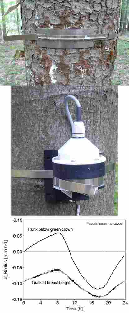
Diurnal changes of tree water storage and stem growth
The resistance of trees to drought depends among other factors also on the amount of water stored in their tissues. This can be detected using dendrometer data, ideally when combined with sap flow results. The amount of stored water can be estimated when calculating differences in diurnal records of transpiration of foliage and sap flow at the stem base when all data are expressed for the whole tree ([50], [66]). The curves are usually slightly (minutes to hours) shifted, although minimum values were sometimes observed even in large trees ([21]). The difference between them is negative in the morning when the storage is being depleted and positive from the afternoon until the next morning, when the storage is being refilled (Fig. 36, upper panel, showing one day in early August). The daily cumulative values of the calculated flow differences (Cum_dQ) are parallel to the diurnal courses in stem volume. Diurnal changes in stored water cause pulsing behavior of tree trunks due to the shrinking and swelling of soft stem tissues (phloem and young xylem), and this is visible on diurnal records made by sensitive dendrometers (Cum d_volume). These changes are small (approximately 0.1 to 0.2 mm) when expressed in terms of stem radius, but when considering the size of the entire tree, they may represent units or tens of liters per day (Fig. 36, middle panel). Notice that each of the 2 variables has its own scale. The “dendrometer volume” curve is shifted behind the “sap flow volume” curve by up to several hours. The daily amplitude of stem shrinking was approximately 5.8 dm3 (10.5 - 4.7 = 5.8 dm3) at the given example. However, dendrometers do not record water stored in rigid tissues, especially lignified sapwood. In these tissues, the daily amplitude of water storage depletion and refilling was greater, approximately 37.6 dm3. Therefore, the amount of water withdrawn from rigid sapwood in the example is 31.8 dm3 (37.6 - 5.8 = 31.8 dm3), i.e., 5.5 times larger than the amount recorded by dendrometers. Water in tree tissues is more easily available for transpiration because it does not pass through tree root resistance. Water storage occurs primarily in the conducting xylem (sapwood) of trunks; storage in other tissues such as leaves is less important. The relationship of the two storage variables (i.e., Cum_dQ to Cum d_volume) is linear most of the day, when the impact of dehydration-rehydration processes prevails during sunny days (Fig. 36, lower panel), but no changes in Cum_dQ occur overnight, when the stem grows (d_Volume changes). The example characterizes the situation during hot sunny weather. Dehydrating and rehydrating phases are linearly related. During periods of growth, the tissue water content does not change, but tree volume does, as already differentiated cells are enlarged of as they are hydrated. This process only occurs during the night under good weather conditions. Under rainy conditions, growth can continue over a longer period of time. Insufficient water storage can result in increased tree mortality. This may occur in spring after dry and cool winters, particularly in shallow soils. Water may become inaccessible during long, severe frosts or when the whole tree storage is depleted during warm winters. Seasonal episodes of trunk growth are sufficient- ly characterized by band dendrometers ([219], [221]), but diurnal changes can help to elucidate the causes of the measured changes.
Fig. 36 - Tree water storage and its diurnal application for transpiration - depleting and refilling parts of diurnal curves in August 6th (upper panel). The diurnal coarse of the cumulative depletion and refill curves of sap flow and corresponding changes of whole tree volume (middle panel) and the relationship between both mentioned variables (lower panel). Numbers represent hours there.
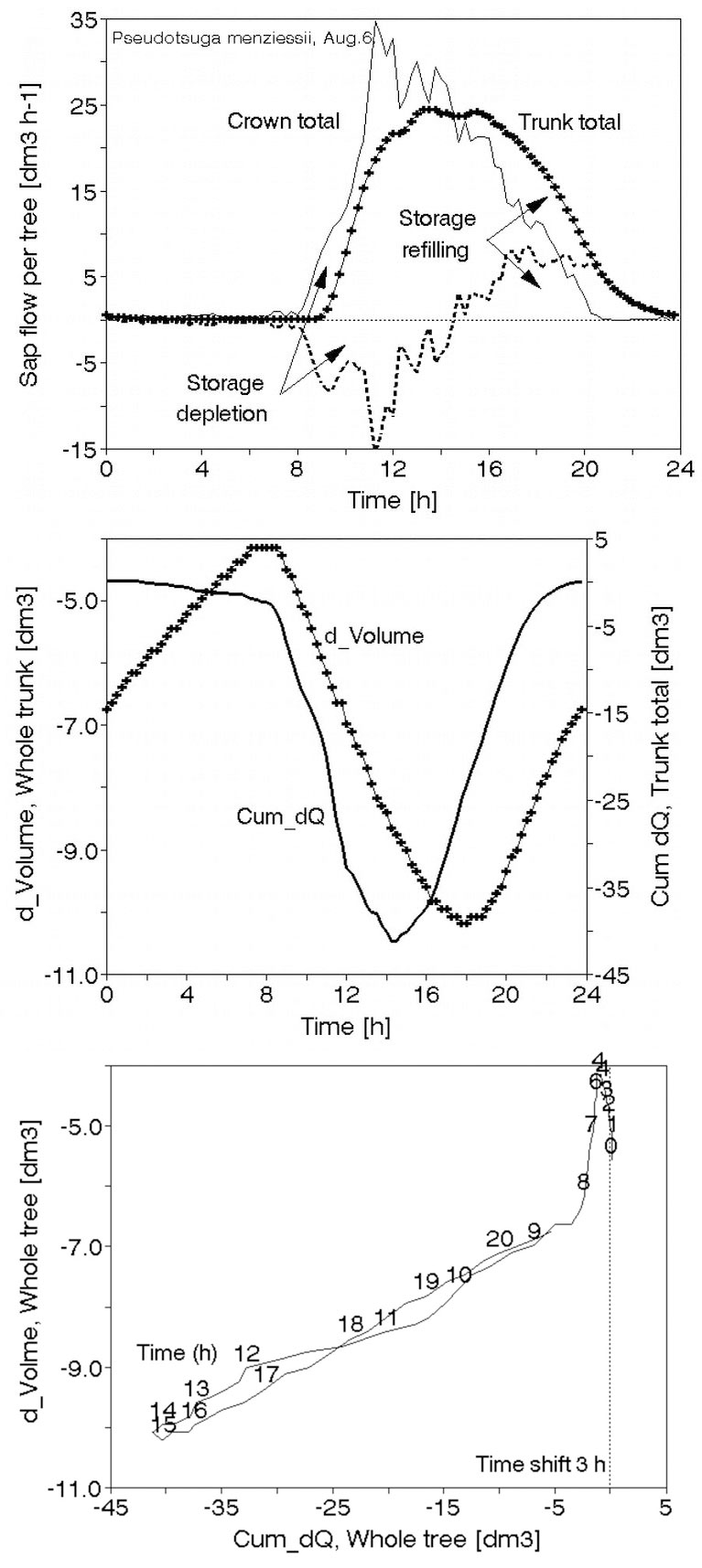
Seasonal changes of stem growth
Annual or seasonal stem growth is probably the most frequently studied process in forestry. Usually institutions for forest management etc. are based on this valuable data source on the large scale (usually national), providing crucial information about timber production and yield. Plenty of literature is available in this scientific field. Therefore we avoid detailing information about this notorious topic, only a small example is used to illustrate this issue. An example of seasonal changes of stem radius in pedunculate oak (Quercus robur) confirms that the available models are capable of precise work. The model results are mostly very well confirmed by direct measurements (Fig. 37 - upper panel). This is true for situations when tree volume increases during growth as well as when tree volume decreases due to tissue shrinking e.g., usually due to drought (Fig. 37 - middle panel). There are good possibilities to get a better understanding of the growing processes, when comparing such data with sap flow rate, or relative transpiration or effective crown area, etc., which can significantly help to evaluate water supply conditions including drought or lack of aeration causing hypoxia (Fig. 37 - lower panel).
Fig. 37 - Example of seasonal growth of stem radius in oak (floodplain forest Lednice, southern Moravia - [219]). Simulated data (especially visible in periods with interrupted records) well correspond with measured ones (upper panel). Actual growth and a period of shrinking due to strong water deficit are compared with relative transpiration rate (daily sap flow, Qw divided by potential evapotranspiration, PET - middle and lower panel).
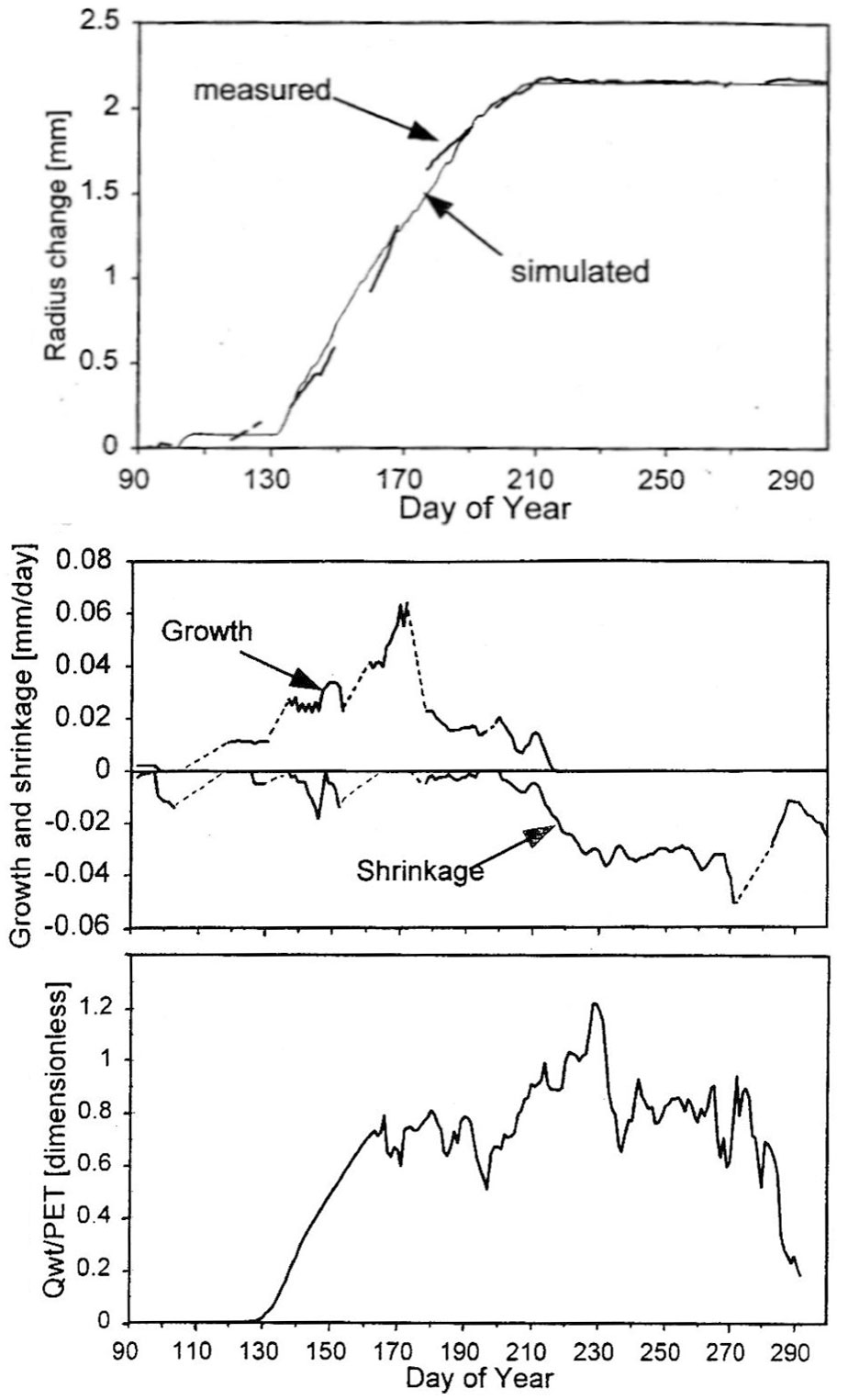
Detection and quantification of water stresses [11]
Usual ranges of transpiration
The approximate range of sap flow or transpiration occurring in the floodplain forest (mostly Quercus robur, Fraxinus excelsior and, to some extent, Tilia cordata) reaches approximately 250 to 450 mm over the growing season or 30 to 600 liters of water per day in individual trees ([50], [40]). The lower values were obtained during a period of time when floods were suppressed by water management measures. In a spruce plantation, the values reached 150 to 250 mm (approximately 10 to 160 liters) per day in individual trees ([220], [221]) The highest transpiration rate, up to approximately 1000 liters of water per tree per day, was observed in willow (Salix fragilis) polycormons with typical spherical crowns growing in a wet meadow near a pond. Thirty-five willow trees situated there transpired per hectare, the same amount of water as grass on the same area ([51]). Stand transpiration was measured continuously at several sites (floodplain forest, spruce plantation and others) for 10 to 15 years over a period of 30 to 40 years (e.g., [62]). A modeling study that also included other data sources, including historical searches, permitted an evaluation of the historical situation several hundred years ago ([186]).
Transpiration data themselves can be sufficient for some purposes, but sometimes it is better to express them in relative terms, e.g., as precipitation (when longer periods of time are considered) or as potential evapotranspiration (over short or long periods of time). Values of the relations to precipitation lo-wer or higher than 1 (=100%) can indicate drought or excessive water. We observed a range from 11 to 253 % in 11 species and 22 different sites (forest types - [46]). Mean values of the ratio of transpiration to potential evapotranspiration reached about 72 % (range: 30 to 96 %) when daily maxims were considered and 43 % (11 to 90 %) when seasonal totals were taken into account. However, transpiration values measured in the above mentioned willows were substantially higher than the potential evapotranspiration. This apparent discrepancy occurred because global solar radiation measured in the usual way on a flat horizontal disc was introduced into the Penman equation. This indicated, that it is not possible to apply global radiation this way, especially when working with solitary grown or dominant trees with open crowns, circumglobal or similar “spatially defined” radiation should be applied. Therefore the effective shape of tree crowns has been introduced ([31]) as discussed later.
Seasonal declines in transpiration (sap flow) in trees due to drought
Because sap flow in trees is very sensitive to changes in environmental conditions, it can be used to diagnose a variety of stresses, particularly drought and hypoxia, but also defoliation, e.g., caused by insects, or root damage caused by fungi. Under conditions of sufficient water supply, the seasonal curve of transpiration in broadleaved species roughly follows that of solar radiation. The impact of severe drought stress is manifested as a dramatic decrease in transpiration during the growing season. The situation under drought is illustrated by examples of shallow-rooting birch (Betula alba) and deep-rooting oak (Quercus petraea - both root depths were measured) that were growing near each other and that were measured continuously for 5 years (Fig. 38, upper panel - [43]). The seasonal amplitude of both species was normalized to the maximum value. Transpiration (or sap flow rate, Qw) depended on leaf development, which began in late April and persisted to late October. During sufficiently moist years, minimal differences were observed in the seasonal courses of transpiration of the 2 species. However, severe drought, which occurred as early as June of the third year of the study, caused a dramatic decline in transpiration in birch.
Fig. 38 - Impact of drought and hypoxia on sap flow rate in trees. Seasonal and diurnal courses of sap flow, Qw in birch (Betula alba) and oak (Quercus petraea) sample trees (enveloping curves corresponding to fine weather conditions) and global radiation Rg (characterizing phases of the growing season) during good soil water supply and drought- (upper panel). The numbers in circles characterize positions of days with the same daily total sap flow, but under sufficient water supply and severe drought ([43]). The diurnal curves are from such days too. Diurnal courses curves are round in springtime under sufficient soil water (day 1 to 4) asymmetrical flattening of diurnal courses from drought stressed days is visible (day 5) as well as the final appearance of stomatal transpiration (peaking in morning hours, day 6 - middle panel). The lowest graph depicts the diurnal courses of sap flow in an ash tree (Fraxinus excelsior) growing in the floodplain forest at the edge of flooded and not flooded part of stand. Measurements were taken a week after flooding, whereby part of roots occurred below the water level, i.e., under conditions of very poor air supply (hypoxia) and the rest in rather wet, but still partially aerated soil (lower panel).
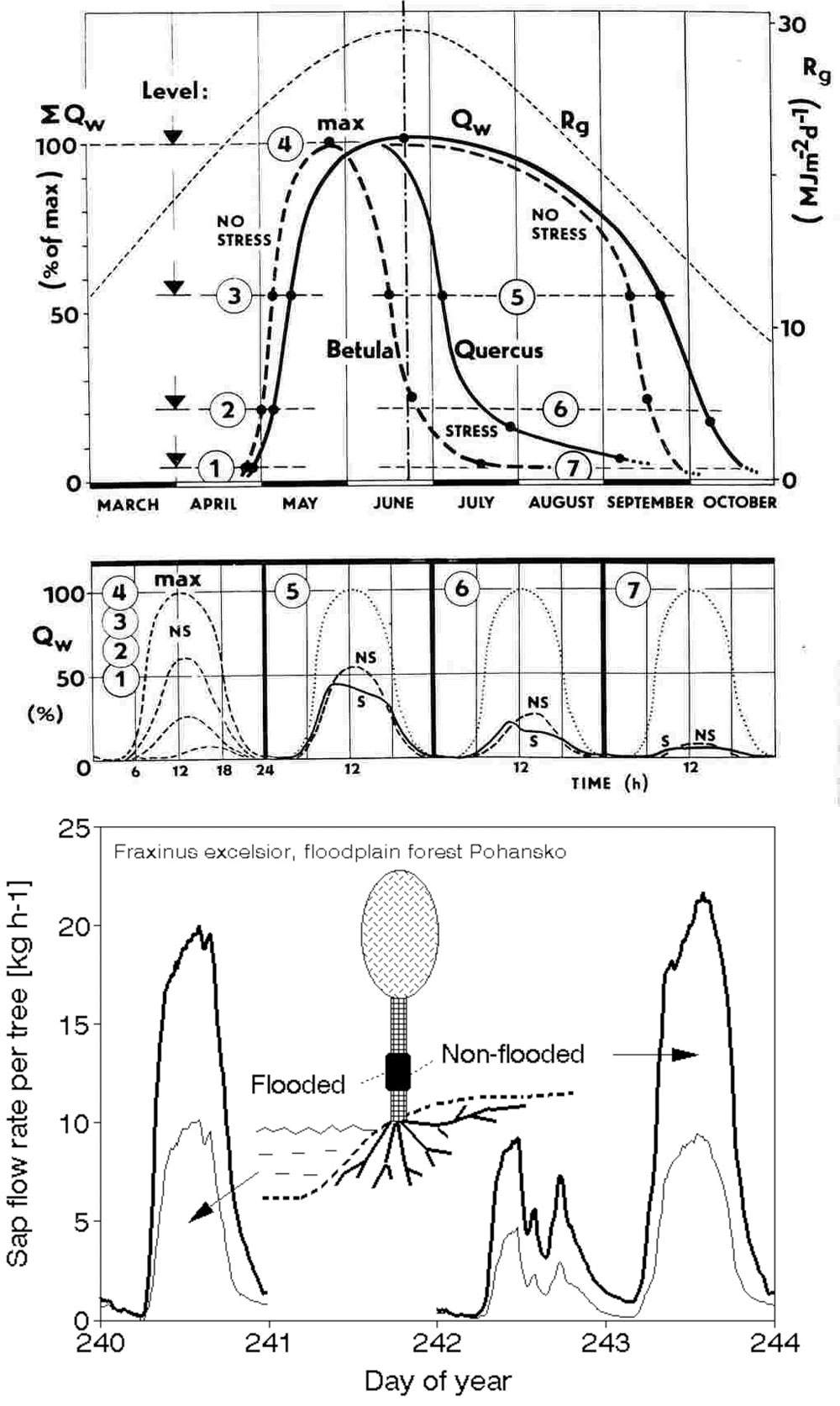
Diurnal declines in transpiration (sap flow) in trees due to drought
Diurnal courses of sap flow are usually symmetrical and have a round form during good soil water supply (for an example, see the first series of 4 days, when the soil was still wet after winter (Fig. 38, middle panel- [43]), but change dramatically during stress. Drought usually causes gradual asymmetric slanting and flattening of the midday and afternoon part of the diurnal course (in the example, note days marked by the numbers 5 to 7 and their positions at the seasonal curve; the dashed line shows non stress days, and the full line shows stress days with the same daily total). The amplitude of sap flow decreases at the same time (see day 5). Differences between the linear parts of the course during the morning and afternoon correspond to decreases in soil water that occurred within this period of time. A day with a small morning peak is occasionally observed, which indicates the last occurrence of stomatal transpiration (see day 6). When the diurnal curve decreases as much as is shown on the last selected day (day 7), the impact of drought on trees is different, as occurred during late September/ October and in mid-July. In July, the occurrence of such a situation usually causes rapid browning of leaves and tree decline. The observed early decline of birch trees brought about by drought was clearly caused by insufficient soil water storage, which affected trees rooted in shallow soil. In oaks, transpiration continued without any sign of drought impact during the entire growing season during the first year of drought because the oak tree, with its deep root system, uses a much larger soil volume. Unfortunately, the drought continued the next year, during which the transpiration of oak trees decreased almost as much as transpiration in birch had the previous year. Luckily, the oak tree survived. However, it may take years for the deep soil water storage to be refilled.
Decline of transpiration (or sap flow) caused by hypoxia
A similar decrease in the sap flow rate occurs in trees under low soil aeration conditions that cause root hypoxia (such as during prolonged flooding - Fig. 38, lower panel). This can also lead to tree decline. However, in this case, there is no flattening of the diurnal curves; their amplitudes only rapidly decrease, indicating that roots situated in better-aerated soil can function normally. Diurnal courses indicate problems before they become critical, allowing sufficient time for instituting protective measures such as artificial stimulation of water outflow from flooded areas by trenching.
Both the above-described changes in seasonal and diurnal sap flow dynamics help to explain the observed growth patterns of trees, especially when considering root systems simultaneously, as well as the general behavior of various species of trees in mixed forests. If the situation is known, appropriate measures can be taken (e.g., watering in parks, implemented thinning), and trees and forests can be protected.
Stand water balance
Sap flow rate data can also be used to calculate tree or stand water balance. This represents a more demanding type of study in which a series of variables must be measured (Fig. 39, upper 5 panels). In the given example, which is from a floodplain forest, letters marks individual items of water balance. The width of the arrows indicates the magnitude of the corresponding water flow in mm (Fig. 39, lower panel). This forest, which grew on a 1- to 2-m-deep layer of heavy soil over an 8-m-deep layer of sandy gravel, relied on an underground water supply under normal conditions during periods of regular floods (4 to 12 times annually, involving snow melt and heavy storms) for up to 70% of its water supply during the growing season This happened when the underground water level moved between 1 and 2 m (or above ground, when water came out of the river bed). However, the situation changed dramatically after water management measures (canalizing the nearby Dyje River) were implemented. The water level then decreased by 1 to 3 m down to the sandy gravel, becoming hardly accessible by roots, resulting in a decrease in transpiration by the dominant trees of 50%. Frequently, shrubs up to 6 m tall (mostly Cornus sanguinea) and herbaceous plants from the understory began to decline. This was followed by the decline of dominant tree species (pedunculate oak, European ash and small-leaved lime) of lower social positions from the main canopy. These types of trees are considered to have unbalanced structures, that is, to possess a relatively small enveloping root area in proportion to their sunlit leaf area. Soil hydraulic conductivity became decisive in this situation. When volumetric soil water content decreased by approximately 4%, soil water potential decreased significantly by 8 bars; however, the hydraulic conductivity decreased much more dramatically, by 100-fold! Under these conditions, trees started to decline. The highest mortality rate occurred in trees with poorly developed root systems or small root area/ leaf area ratios ([40], [41]).
Fig. 39 - Pictures characterizing more complicated instrumentation for stand water balance studies (five upper panels). General scheme of the detail water balance of a floodplain forest composed mostly of oak ash and lime (Quercus robur, Fraxinus excelsior and Tilia cordata) (expressed as a tree - [40], [41]). This was calculated for actually rooted soil volume and supplementary volume (sup), where roots of dominant trees do not occur (only roots of shrubs and herbaceous plants were there). Arrows mark different flows of water, their width symbolizes amounts of water [in mm]. P = precipitation, E = evaporation, Epot = potential evapotranspiration, Eact = actual evapotranspiration, ET.act = transpiration of dominant species, dW=soil water storage, H = horizontal transport, K = maximum soil hydraulic conductivity (lower panel).
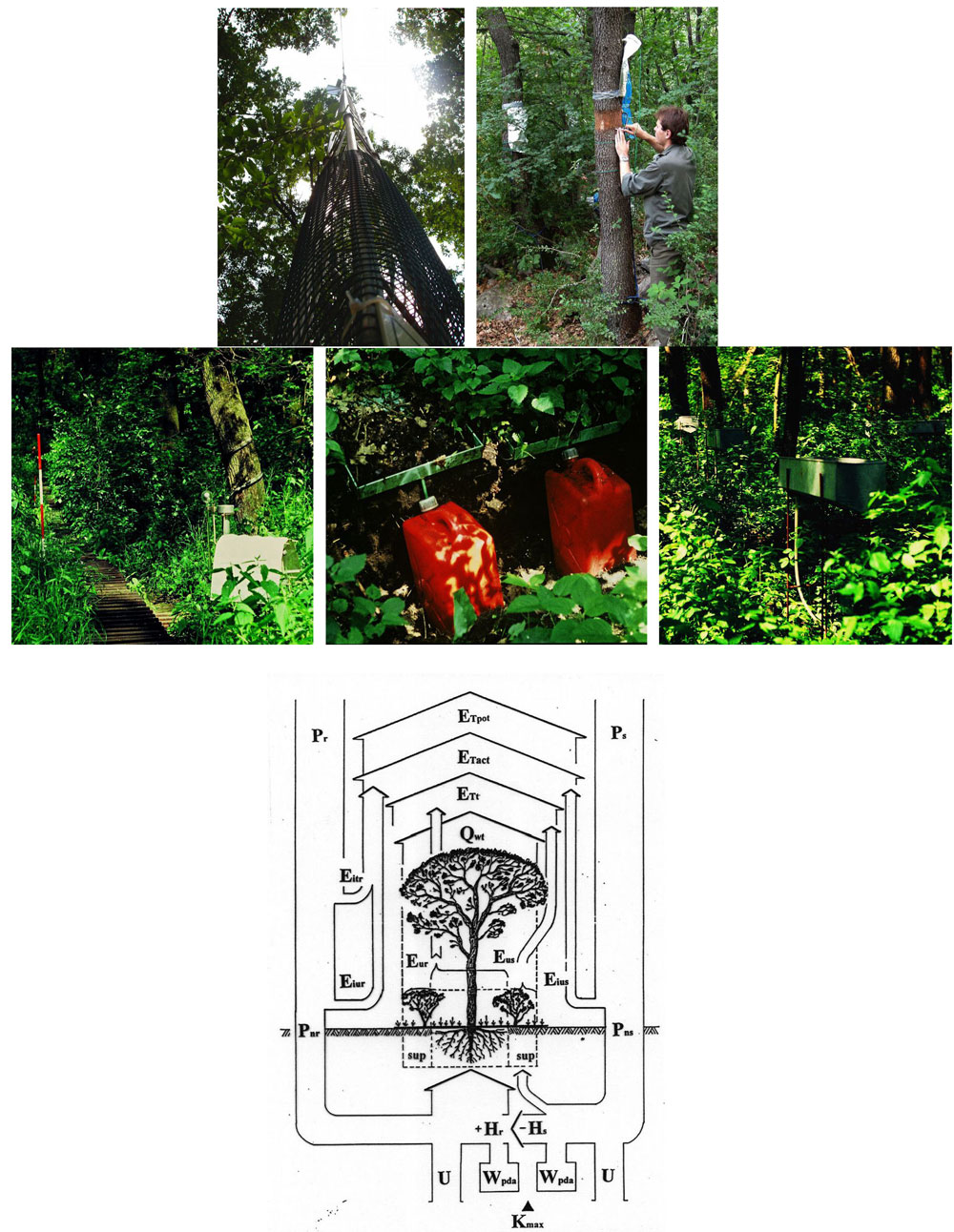
Water redistribution between roots and soil
Although water most frequently moves upward from roots to foliage, in principle, it can move in any direction through the conducting system of trees. The direction of water movement (Fig. 40) depends on the water potential gradients. Changes in the direction of flow therefore depend on the local soil water supply, which can differ significantly in soil layers at different depths ([169], [171], [79]) or if water storage is highly asymmetrical around the tree ([168]). Deep soil layers can supply water to shallow soil layers via tap or sinker roots under drought if they contain more water. Superficial roots can spread this water around trees and partially simulate watering of shallow soil layers (this mechanism may allow survival of herbaceous species around trees, which could not grow there without them). Water is absorbed by superficial roots after rain and transported to the main stem and subsequently to foliage for transpiration. However, if there was previous drought, a part of that water flows down to sinker roots (normal acropetal direction of flow is reversed), of which it can come to surrounding soil if its water potential is lower - recharge of depleted reservoirs appears. Under the coming drought, water is supplied by superficial roots only for a short period of time, because storage in the shallow soil layers is easily depleted. Water uptake then gradually changes and becomes dependent on sinker roots absorbing water from deeper soil layers, until their water storage is available. Some of this water goes to the main stem under such conditions, but the rest goes in the opposite direction to the superficial roots under conditions of low evaporative demands. The mechanism of hydraulic redistribution protects individual roots from decline and consequently prevents the decline of the whole tree. If there is anastomosis between trees, water can move from the root of one tree to the root of the neighboring tree ([172]) and eventually a certain amount of water can move upwards on slopes.
Fig. 40 - Scheme of water redistribution between roots and soil and roots themselves under different weather and soil moisture conditions, which can be easily detected by sap flow measurements. Water in shallow soil layers is depleted first under drought; therefore roots start absorbing water from deeper layers (if available there). This water goes up and than share: part into stems and part into more stressed shallow roots. This is happening in all such roots, so in certain parts of horizontal roots water flows in two opposite directions. Some water from roots can be taken by dry soil, which enables other plants to live there. Water come first to shallow roots after rain and is then supplied by sinker and taproot into deeper soil layers.
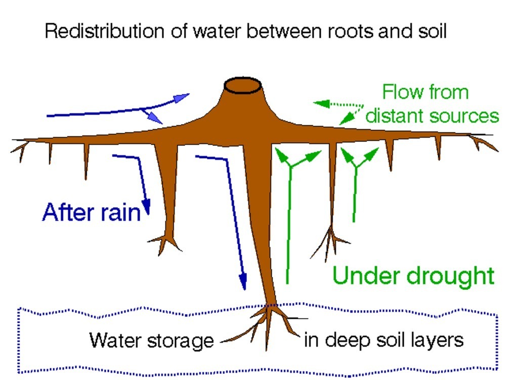
Very interesting sap flow dynamics occurred in small roots during long-term monitoring of their functionality as it is shown for cork oak roots (Fig. 41). Sap flow in all roots changed synchronously according to climatic conditions when soil water was easily available after a wet winter. However, when drought came later, night root sap flow dramatically changed and become asynchronous between different roots: flow gradually increased in some roots (particularly in r3), but rapidly decreased in others (r2), reaching substantial and stable reverse flow from mid June to September, until the first high rain event occurred. Water availability in the surface soil layer increased after the rain. This caused an immediate turn of the reverse flow pattern back into a positive one, similar to the flow pattern which occurred in the spring. The moment when the reverse flow is recorded in the roots (marked by arrows in Fig. 41) indicated the start of hydraulic redistribution through the root. This change also indicated soil drying in places, where particular roots occupied corresponding soil volume. The period of occurrence of reverse flow and its magnitude provides an idea about the depth of individual roots when analyzed together with microclimatic parameters: r2 was a very superficial root, while three others (r1, r4 and r5) grew deeper and r3 was the deepest. Root characteristics described here using sap flow rate data were confirmed after root opening by the supersonic air stream at the end of experiment ([167]).
Fig. 41 - Conducting xylem in stem at breast height is usually very sectored and connected with roots only from corresponding side showing strong segmentation of flow especially in outer xylem. If large root would be cut below sensor installed at stem base, then sap flow radial profile will indicate abrupt flow decrease (see left upper panel with example of sap flow radial pattern measured by the HFD sap flow sensor at breast height before (black) and after (red) root cutting below the sensor). In trees with prevailing sectored hydraulic architecture no changes would be recorded from the opposite stem side just below crown. But in trees with prevailing integrated hydraulic architecture flow spreads and overlaps with height of tree and conducting xylem in stem just below crown is connected with roots from all sides. That is why damage of one even big root could be not so crucial to the whole crown (see right upper panel with example of sap flow radial pattern measured by the HFD sap flow sensor just below crown just before (black) and after (red) root cutting from the opposite stem side). High heterogeneity of root distribution around stem very often causes high circumferential sap flow variability, which became much lower with height of tree. Branch cutting with synchronous measurements of sap flow in stem could be also similarly used to study tree hydraulic architecture (according to [169]).
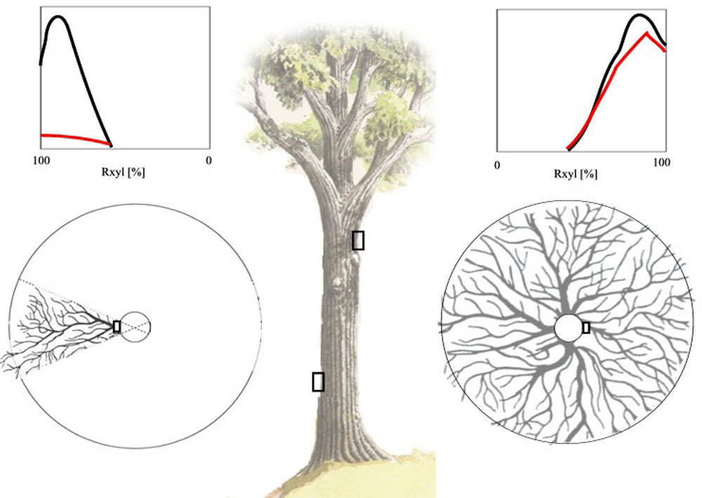
Neglecting hydraulic redistribution mechanism may cause great practical problems. For instance, an owner of a huge tea plantation in a dry part of Kenya supposed that Acacia trees growing at the same plantation are competing for water with his favorite tea. He did not consult this issue with specialists and ordered the removal of all Acacias. Unfortunately, this was followed by a massive and immediate decline of tea plants and the whole plantation was destroyed to his great surprise (Jan Pokorný, personal communication).
Hydraulic redistribution in branches
In addition to soil-root-stem water movement, water can also be redistributed between different branches in the tree crown. When tree tissues normally rehydrate overnight, redistribution of water is most pronounced in the morning after the crown is irradiated from the east. Water is then redistributed from west facing to east-facing branches, especially in species with sectorial conducting systems. Similarly, redistribution continues over different azimuths throughout the day according to changes in the tree crown radiance due to the “rotating Sun” ([77], [215], [169], [171]).
The tree conduction system and its hydraulic architecture
The conduction systems of coniferous and broadleaved trees are highly variable and depend on the type of grain present, which may be sectorial, spiral, zigzag or integrated, among other possibilities ([200], [199], [122], [169], [78]). In addition, the grain of the tree can change to some extent during the tree’s life, complicating studies of tree behavior. If a single root is damaged in trees with sectorial straightforward conduction system, most branches growing above it will not be supplied by water and therefore will die. If a similar root is damaged in trees with integrated conduction system, transporting water to all branches in the crown, total transpiration will decrease slightly, but no branch will die. This occurrence is therefore important from a practical perspective. In the above-cited and other related studies (including measurements of stem cross-section profiles of sap flow), Cermák et al. ([56]) described these phenomena via anatomical analysis on the basis of xylem staining, which inevitably led to tree destruction. However, current sap flow measuring methods, especially the HFD method ([163], [170], [78]), which uses multipoint sensors ([30]), permit the characterization of conduction systems in a similar way as in stem cross-section studies (see the corresponding chapter) without destroying the tree. Heterogeneity of the root distribution around the stem very often causes large variations in circumferential sap flow that decrease dramatically with stem height. For example, the measurement of sap flow from 2 opposite sides of the stem of European larch revealed very similar rates, and these decreased only slightly below the crown, reflecting the prevailing sectorial grain of the tree. By contrast, sap flow at the stem base in Norway spruce differed substantially around the stem but became much more uniform below the crown, indicating this species’ integrated hydraulic architecture ([202]). The conducting xylem present in stems at breast height is usually sectored and connected with roots, presumably those growing in the same direction, particularly when considering the outer xylem (Fig. 42, left circle and panel). If a large root would be cut below a sensor installed at the stem base, then the sap flow radial profile would indicate an abrupt flow decrease (see left upper panel with example of sap flow radial pattern measured by the HFD sap flow sensor at breast height before (black) and after (red) root cutting below the sensor). In trees with prevailing sectored hydraulic architecture no changes would be recorded from the opposite stem side just below the crown. But in trees with prevailing integrated hydraulic architecture the flow spreads and overlaps with height of tree and the conducting xylem in the stem just below the crown is connected with roots from all sides. That is why damage of even one big root could be not so crucial to the whole crown (see Fig. 42, right upper panel with example of sap flow radial pattern measured by the HFD sap flow sensor just below crown before (black) and after (red) root cutting from the opposite stem side).
Fig. 42 - Responses of sap flow in large Quercus suber tree to branch severing. Dynamics of sap flow measured from two opposite stem sides (NE and SW) and sub-branches of two large branches situated above each sensor were gradually cut with a certain time interval between cutting to allow clear responses to be detected. Full vertical lines indicate moment of cutting of sub-branches of NR branch and dashed lines of SW branch respectively. It is well visible, that each sensor reflected by flow decrease only on cutting sub-branches above it (see [78]).
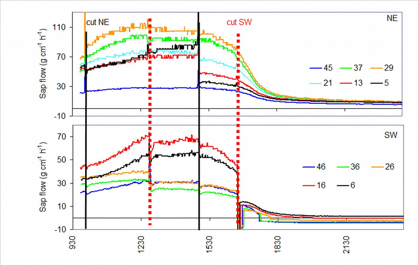
Branch severing with synchronous measurements of sap flow in stem could be also similarly used to study tree hydraulic architecture. More information can be obtained using very short recording periods (minutes or seconds). An example of such an experiment involving a large oak tree (Quercus suber) is shown. Multipoint sap flow sensors were applied at the trunk base, and branches were subsequently severed over a period of several days in such a way that several small branches were cut from the large first-order branches (to observe flow responses separately, see Fig. 43). Flow records from only 2 sensors at the opposite trunk sides are shown; responses of flow only from the side on which branches were situated were visible. The experiment allows studies of connections through stem xylem between different parts of the tree skeleton - branches or roots. It confirms that oak has a pronounced sectorial structure such that sap in a certain part of the trunk flows only to the branches above it ([78]).
Fig. 43 - Nighttime dynamics of sap flow in five small (2nd order) roots of cork oak tree (Quercus suber) measured over the entire growing season (March to September). Sap flow in all roots changed synchronously according to climatic conditions when soil water was easily available after a wet winter. However, when drought came later, night root sap flow dramatically changed and become asynchronous between different roots: flow gradually increased in some roots (particularly in r3), but rapidly decreased in others (r2), reaching substantial and stable reverse flow from mid June to September, until first high rain event occurred. Water availability in the surface soil layer increased after the rain. This caused an immediate turn of reverse flow to positive flow, similarly as t in the spring. The initiations of reverse flow in the roots (marked by arrows) catalyzed the start of hydraulic redistribution through the roots. It also indicated soil drying in places, where particular roots occupied corresponding soil volume. The period of occurrence of reverse flow and its magnitude gives an idea about the depth of individual roots when analyzed together with microclimatic parameters: r2 was a very superficial root, three others (r1, r4 and r5) were growing deeper and r3 was the deepest. Root characteristics described here using sap flow rate data were confirmed after root opening by the supersonic air stream at the end of experiment ([167]).
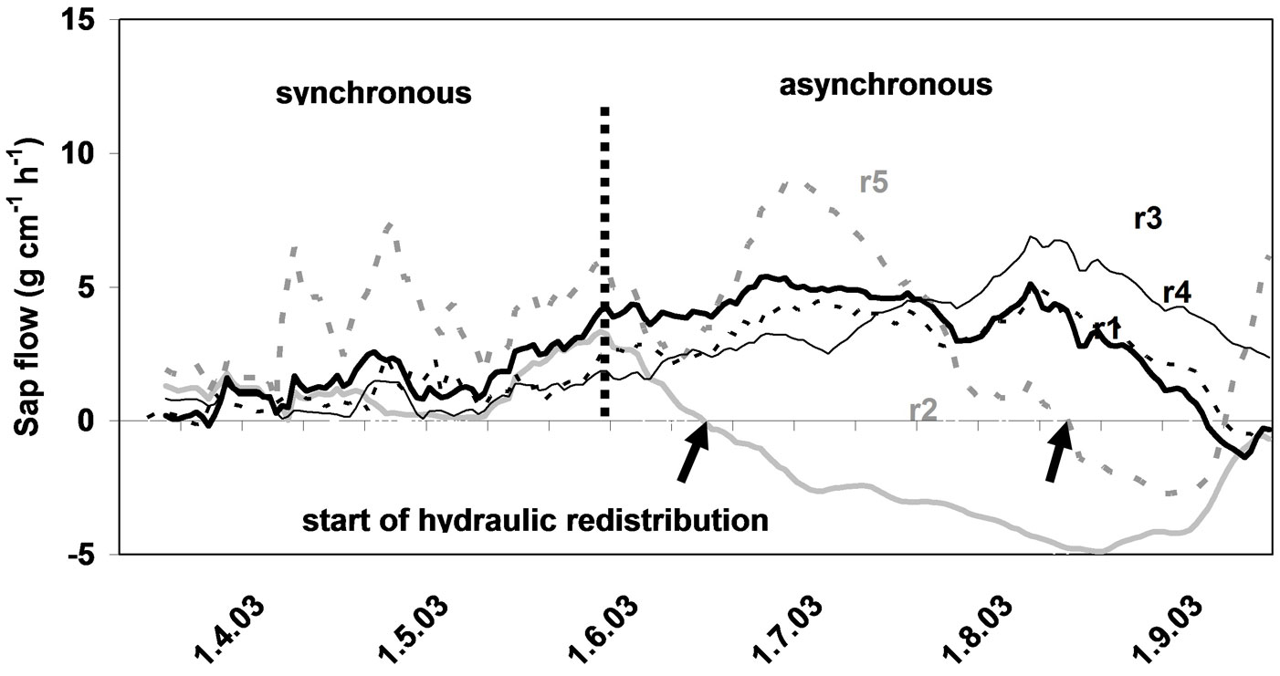
Experimental treatment of trees using sap flow [12]
Impact of actual soil moisture and permanent damage to conducting systems
The impact of actual soil moisture and the occurrence of permanent damage to conductive systems (e.g., due to vessel emboli or plugging by thylls, decrease in leaf area) can be distinguished by diurnal changes in sap flow amplitude after localized soil watering. Such a situation in a 115-year-old mixed forest (mostly Fagus sylvatica, Fraxinus excelsior, Abies alba, Picea abies and Pinus sylvestris) growing on a mountain plateau with heavy soil in Switzerland ([144], [57], [58]) is illustrated in Fig. 44. The site was wet at the surface every spring but always became very dry in late summer. The forest was seriously damaged by wind (50 % of trees removed); this was followed by rapid beech tree decline but not by the decline of any other species. The declining beech trees were those originally growing in the denser parts of the stand. These trees were partially shaded by their neighbors and were able to meet their water requirements for transpiration by means of relatively small root systems. These root systems were smaller than the projected areas of their often-asymmetric crowns, the branches of which had a tendency to grow into more open parts of the canopy. The projected root area of these trees was visible from the pattern of the undergrowth (0.5 to 1 m tall), which was completely missing in circles approximately 5 m in diameter around damaged trees (only bare soil covered by litter occurred there), while it was very dense elsewhere at the site. The remaining healthy beech trees were situated in more open parts of the canopy, and their root systems were significantly larger than their projected crown areas. Thus, they were more resistant mechanically and physiologically because they had much larger volumes of soil at their disposal (Fig. 44, upper panel). Healthy trees transpired substantially more water than trees that were damaged. Healthy trees also responded very little to localized irrigation, while the responses of damaged trees were pronounced, when a car with a 500 liter barrel came to the site (Fig. 44, middle panel). In the damaged trees, the sap flow rate increased exponentially after 2 subsequent irrigations (50 mm each), but there was no response after a third irrigation (Fig. 44, lower panel).
Fig. 44 - Experimental design (watering system and a series of sample trees in the mixed forest (upper two panels). Diurnal course of sap flow in healthy and seriously damaged beech trees (Fagus sylvatica) during repeated localized irrigations (lower panel). An arrow marks the onset of each irrigation. (Sap flow measured 4 m above ground responded to irrigation 6 minutes after the first drop of water touched the ground) and subsequently three times within about 4 hours (modified after [144], [57], [58]).
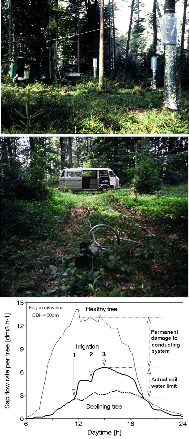
The amplitude of the diurnal curve of the damaged trees was 3 to 4 times lower than that of healthy trees, and it roughly doubled after irrigation, when the soil water supply became non-limiting. However, the amplitude of the diurnal curve still remained much lower than when the trees were healthy, indicating a level of permanent damage to the trees’ conductive systems. The differences in sap flow rate between the non-irrigated and fully irrigated states (indicated by a lack of response after irrigation) in the damaged tree characterize actual soil moisture limit. The difference between the fully irrigated state in the same tree and its healthy neighbor indicates the level of permanent damage to its conducting system (including embolized vessels, smaller leaves, etc.). On this basis, we recommend that local foresters should maintain sparser forest from the beginning so that each individual tree occupies a larger stand area and becomes more resistant to mechanical (wind) as well as physiological (drought) disturbances.
Automatic irrigation control based on sap flow index
Sap flow measurement can also be used in conjunction with automatic watering, i.e., mist irrigation control of tree water status, for instance, in orchards. The symmetrical temperature difference dTsym within the HFD sap flow sensor, also known as the sap flow index (SFI), may be used as a stress indicator ([159], [161]). Alternatively, SFI can be measured using a very simple sensor with three precisely fixed needles in which the middle needle is a heater and the two other needles, which are thermocouples, are displaced equidistantly around the heater in the axial direction ([157]). The temperature difference dTsym represents one of the raw signals in the HFD method for sap flow measurements and characterizes the axial deformation of the heat field near the linear heater caused by the ascent of sap. On a cloudless day, SFI displays an “unusual” pattern with 2 maxims, 1 in the morning and 1 in the evening, and a midday depression (Fig. 45). During the growing season, predawn SFI values (SFIp) are very variable. SFIp is usually low on a wet day, and it increases to the morning maximum with increasing drought. The midday values of SFI are related to dehydration of the stem tissues due to transpiration. The ratio of predawn to midday SFI is a very sensitive indicator of the plant’s water status; this ratio increases substantially with drought stress. An “air-drought-stress curve” was used to characterize the development of water stress in trees subjected to air drought during the growing season ([157], [159]). This feature was used for automatic irrigation control in an apple orchard ([157], [158], [160]). In addition, the period between the morning and evening SFI maxims (dT) and the difference between them (dM) are important ([158], [160], [161]). With increasing water stress, the period between the SFI maxims increases, whereas the difference between their values decreases. Night and, in particular, predawn tree water status is an important indicator of drought stress in trees. Leaf water potential is frequently used as a measure of tree water status and drought stress; however, there are difficulties associated with sampling foliage from tall trees and determining leaf water potential automatically. By contrast, SFI can be automatically and continuously recorded even during very low flows and can be used to estimate tree drought stress caused by dry air under no limiting soil water conditions.
Fig. 45 - Typical daily curves of sap flow index (SFI) measured in tree stems onwet (upper panel) or dry (lower panel) days. Three different characteristics of the daily SFI curves may be used as stress indicators: the difference between the morning and the evening maxims (dM 1.2), the period between both SFI maxims (dT) and the ratio of SFI measured at predawn (SFIp 1-2) to its midday value (SFId - from [168]).
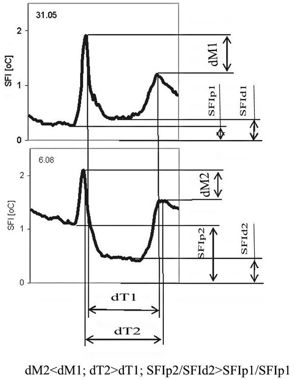
Detection of underground root damage caused by heavy machinery
Heavy machinery such as lorries or trucks is usually used for transporting large amounts of materials. If transport occurs on hardened roads or highways, nearby trees can be jeopardized by accidents, but usually few roots grow beneath constructed roads. However, the situation is quite different when heavy machinery, particularly tractors or harvesters, is used directly within forest stands. Mechanical damage (e.g., rubbed-off bark and smashed outer wood) is clearly visible on the lower parts of stems and on coarse roots at the ground surface. Unfortunately, similar or even more serious damage to underground root systems is not visible, and therefore, it is systematically neglected. Nevertheless, several of the above-described measuring systems can be used to detect mechanical root damage. Ground-penetrating radar and acoustic pulsing are suitable for coarse root studies, modified earth impedance and sap flow vectors can be used for fine root studies, and the supersonic air stream technique can be used to verify the results obtained. Both of the above-mentioned methods for coarse root measurements can visualize large-scale damage to root systems, which does not occur very often. The fraction of absorptive fine roots that are situated exactly below the tires is relatively small compared to the whole root systems of the sample trees; this fraction of the roots is usually smashed or broken, but it can regenerate if the soil conditions remain suitable after treatment. When coarse roots are damaged, most roots that supply water to trees or serve as sinks for assimilates become dysfunctional; therefore, this type of damage is more serious.
Sap flow study in roots treated by heavy loading (Fig. 46) demonstrates root responses ([166], [172]). Loaded tractors or harvesters moved along skidding lines, where many (altogether 90) sap flow sensors were installed on tree stems and individual roots. Movement of each tire across coarse roots was visible on the sap flow records, first as a significant flow increase (when it was pushed in roots by heavy weight), but than followed by flow decrease, when tracheids in the upper parts of root conducting xylem were smashed and interrupted. This fit for roots occurring in the upper soil layers down to the depth of about 15 cm, when the tire moved closer than 1 m distance from stems ([166], [172]). No healing of wounds caused by passing of loaded tires above roots was found the whole year after root treatment ([85]), therefore such wounds could serve as infection points for fungi, which represents a greater threat to trees than direct mechanical damage.
Fig. 46 - The example in the study focused on tree root damage caused by movement of heavy machinery along skidding trails in a shallow rooting species (Norway spruce). The upper right panel shows a loaded harvester moved along a skidding line. A sample spruce tree with installed HFD sap flow sensors in the roots and in the main stem is portrayed just at the moment when it is loaded by passing forwarder tires (upper left panel). Examples of sap flow responses upon loading are included. Periods of loading are marked by dashed vertical lines (lower left panel - [171]). Roots were opened by the supersonic air stream at the end of the experiment and were covered by soil again after making photo-images. Open wounds remained serving as places for following fungi attack.
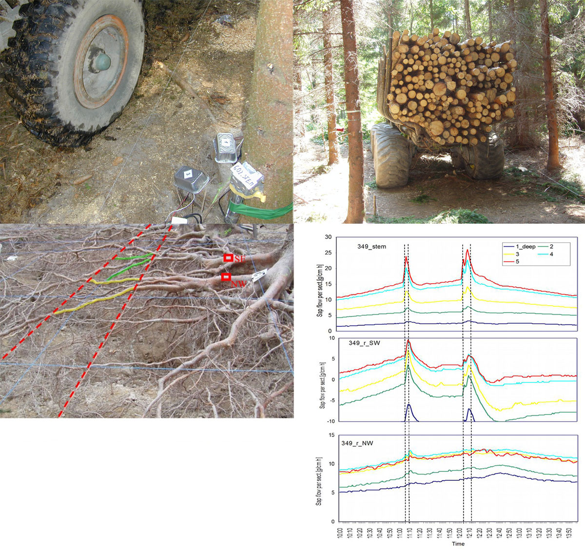
Example of a spruce sample tree with installed HFD sap flow sensors in roots and in the main stem (Fig. 46, left panels) just at the moment when it was loaded by passing forwarder tires (Fig. 46, right upper panel). Examples of sap flow responses on loading. Dashed vertical lines mark periods of loading (Fig. 46, right lower panel). The substantial response of sap flow (first increasing, then decreasing) and its overall final decline is visible in treated root from the SW-side. A very slight response in the outer sapwood layers was recorded also in root 349_NW, although this happened only during the first treatment. There was no reverse flow in the main stem, while it occurred pronounced in the SW root, associated with the close-by anchoring root and indicating water lifting there. No such lift appeared in root NW, where the anchoring root was at a distance.
Functional parameters quantifying whole trees
Simulating sap-flow and related variables in trees and stands [13]
Analysis of water movement
The sap flow pathway can be simulated by using a network (the circuit) at the whole tree level, which can be described in terms of electrical symbols. The sap flows through a network of resistances (R) down a gradient of water potential between leaves (foliage, ψf) and soil (ψs), dψf-s, which represents the suction force (see Fig. 11, lower panel). The soil layers are assumed to act as resistors in parallel; each layer contains soil (Rs) and root (Rr) resistances in series, and Rm characterizes stem and Rf foliage resistances. The large store of water present in stems, which is represented by capacitors (C), acts to buffer sap flow. Sap flow through the resistance network is generated by transpiration (a tree-related part of stand evapotranspiration = water loss E), which is controlled by stomatal opening and aerodynamic resistance.
The vapor pressure difference (in Pa) between the internal leaf spaces (Pf) and the atmosphere (Pa), dPf-a=Pf - Pa, governs the atmospheric water demand. Stomatal resistance is varied to maintain E at a rate that keeps ψf from falling below a critical threshold value (ψf.min), below which potentially dangerous cavitation of the tree hydraulic system can occur. Therefore, when ψf = ψf.min, E is set so that dψf-s/dt = 0, where (eqn. 6):
where the gravitational component of leaf water potential is calculated from the density of water (ρw), acceleration due to gravity (g) and the height above the reference plane (h), which is set to the soil surface. The capacitance (C), is the change in tissue water content (storage, W) for a given change in water potential [C = dW/dψ]; W varies as the difference between the sap flow into the tree (Q, which can be approximately taken as that at the tree base) and the flux out (E), [dW/dt = Q - E]. Therefore, the sap flow at the stem base can be determined from the evapotranspirative losses as Q = E + (Cdψ/dt) ([242], [243]).
Leaf (foliage) specific hydraulic conductance (kf = 1/Rf) can be expressed [mm s-1 Pa-1] from transpiration per leaf area units (kg m-2 s-1 - Ef) and the water potentials as (eqn. 7):
where Ef can be replaced by Ef = kf dPf-a when taking gs as the stomatal conductance.
Potential evapotranspiration
Fig. 47 - Function-based (active physiological) areas. When discussing potential evapotranspiration (PET), we should have in mind a short cut grass lawn (according to Penman’s definition, upper panel), which differs in details from the tree canopy structure (e.g., in pine, middle panel). The effective projected crown area (Act_ef), calculated from the ratio of daily values of tree transpiration (EQ) and potential evapotranspiration (PET) and the theoretical active projected root area (Art_ef), calculated from the ratio of EQ to daily change of soil water content in the rooted zone (dVw). This can be considered, when soil water content is measured by a series of sensors situated around the tree (supposing that values of dVw = 0) characterize the edge of the rooted zone. Act_ef can be taken as a certain value of crown conductance (including crown irradiance in addition to vapor pressure deficit - lower panel).
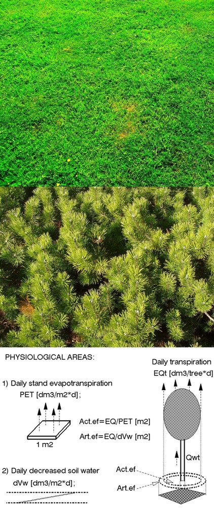
The equation to derive potential evapotranspiration (PET, [kg m2 s-1 = mm s-1]) was first derived by Penman ([181]) for a standard crop (short-cut grass lawn - Fig. 47 upper panel) in the form (eqn. 8):
where Δ is the slope of saturation vapor pressure curve [Pa K-1], Rn is the net radiation [W m-2], estimated as 70% of global incoming solar radiation, D is the vapor pressure deficit (es-ea) during the period [kPa], ea is the vapor pressure of free flowing air and es is the saturated vapor pressure at a given air temperature, γ is the psychrometric constant (taken as 66 Pa K-1), λ is the latent heat of vaporization (24 500 J kg-1) and u2 is the wind speed measured at the height of 2m (m s-1 - it could be taken as a constant 1.5m if not measured). Notice: if taking immediate values insert the Rn in W m-2 and for daily totals in J d-1 m-2.
When detailed input data are not available, PET ([mm d-1]) can be approximated by simpler equation, such as that developed by Turc ([228]). This is based on global radiation and air temperature only, but was recommended by Federer et al. ([83]) as one of the best simple equations (eqn. 9):
where daily total of global radiation Rg is in MJ m-2 d-1 and mean daily temperature Ta in °C (e.g., for Rg = 22.031 and Ta = 22.7, it gives PET = 4.51 mm d-1).
Actual evapotranspiration and crown conductance
Actual evapotranspiration and crown conductance (E, [kg m-2 s-1]) can can best be calculated by the following Penman-Monteith equation (eqn. 10):
where Cp is specific heat of air (J kg-1 K-1), ga is air conductance and gc is canopy conductance (m s-1). However, values of ga and gc differ in a grass lawn and tree crown (Fig. 47, middle panel) and are difficult to measure in tall trees under open field conditions. Therefore some functional parameters of tree crowns, such as relative transpiration (relative to PET) and effective projected crown area, can be useful.
The relation in eqn. 7 is somewhat simplified and does not include the effect of height and similar factors ([145]). A more exact approach is conducted using the inverse form of Penman-Monteith equation (eqn. 10), as follows (eqn. 11):
Crown conductance gc ([m s-1]) related to ground surface area can be calculated from whole tree transpiration rate per unit of ground surface area Ac_pro and ambient vapor pressure deficit D according to the simplified equation ([m s-1], [121] - eqn. 12):
Functional parameters of tree crowns [14]
Effective projected crown area
Projected crown area (in m2 per tree) is one of the most simple and frequently used operative biometric parameters of tree crowns. It includes some errors caused e.g., by individual sparse branches, where it is not sure, whether it is better to include them or not and also because crowns can be of very different shape, lengths and leaf densities. Therefore, we can also calculate at the stand level relative transpiration (EQ/PET in %) and apply the same equation, but expressed per individual trees as the effective projected crown area (Ac_ef in m2 per tree), which is calculated as the ratio of the daily totals of transpiration or sap flow (EQ in kg day-1 tree-1) and potential evapotranspiration (PET in mm day-1, i.e., in kg m-2 day-1 - [50]). We found that this variable well reflected drought stress, which was confirmed also by other authors ([198] - eqn. 13):
This ratio can be expressed as relative transpiration in percentage of PET when working with entire stands or in square meters per tree when introducing values for a single tree ([50]). Ac_eff can be also taken as a certain measure of crown conductance (including crown irradiance in addition to vapor pressure deficit - eqn. 14, eqn. 15). However, using this approach, we assume that tree crowns are flat, similar to a standard plant stand (usually a short cut lawn). Therefore, estimation of the effective form of tree crown is important ([32]). Analogously, it is also possible to derive the effective projected root area (Ar_act), which is calculated from the ratio of EQ to the daily change in soil water content in the rooted zone (dVw - Fig. 47 lower panel). Soil water content is measured by a series of sensors situated around the tree (supposing that values of dVw = 0 characterize the edge of the rooted zone - eqn. 14):
[m2 tree-1] or simplified version according to ([121] - eqn. 15):
[m2 tree-1]. When expressed for canopy conductance (eqn. 16):
[m s-1] or again a simplified version (according to [121] - eqn. 17):
Effective form of tree crowns
Measurement of the geometrical form of tree crowns is too complicated for practical application in forests of different densities and containing different species, but estimation of the effective crown form is rather simple and therefore widely applicable. It is based on a comparison of the diurnal course of sap flow with the course of radiation (eventually introduced into PET) measured at the flat horizontal plane (i.e., global radiation), at the sphere (as the circumglobal radiation) or based on different simple geometrical forms (e.g., ellipsoid, paraboloid). Technically speaking, it is better to apply data obtained during the morning hours to avoid the disturbing effect of the afternoon saturation flows (Fig. 48, upper panel). The diurnal curve of sap flow in the suppressed tree is linearly related to global radiation, whereas the sap flow of the dominant tree deviates from the line (Fig. 48, middle panel). The suppressed tree therefore behaves as if it has a crown with a flat form. The diurnal curve of sap flow in the dominant tree is linearly related to circumglobal radiation, while the sap flow of the suppressed tree deviates from the line (Fig. 48, lower panel). The dominant tree therefore behaves as if it has a crown of spheroid form. Individual trees in stands as well as stand totals can be described using this approach. Stand radiation dynamics-based estimates of the effective forms of forest tree crowns are similar to those based on direct measurements of leaf distribution and estimates of sunlit area. Using this method, we can better characterize the amount of absorbed energy and obtain more precise background information for evaluating stand hydrology and growth effectiveness. The amount of radiant energy absorbed by forest stands depends to a large extent on their optical roughness. Optically flat stands, even when fully leafed (high LAI) and with closed canopies, as demonstrated in the example of beech (Fig. 49, upper panel), are less illuminated from the side and therefore have a smaller sunlit area, while in stands with tree crowns that are spatially more variable, more light penetrates through the gaps, and the daily total of stand illumination as well as the sunlit leaf area are greater (Fig. 49, lower panel). Measurement of crown shape and density is easier in trees with straightforward sectorial conducting pathways, while spiral or zigzag pathways may sometimes cause problems. However, these are presently being analyzed, and the results will be presented shortly.
Fig. 48 - Functional parameters of tree crowns - estimates of the effective crown form. Diurnal records of global and circumglobal radiation and sap flow rate in dominant and suppressed trees (upper panel). Radiation records differ when applying at the flat horizontal sensors (i.e., global radiation provided by most meteorological pyranometers, Rg) or at the sphere of the same diameter (circumglobal radiation, Rcg) or eventually applying any spatially pronounced form, e.g., ellipsoid, parabolloid, conus, etc. Diurnal courses of sap flow can be more similar to Rg (especially in suppressed trees - middle panel); therefore the effective crown form in such trees is approaching a flat horizontal disc. If the diurnal course of sap flow is approaching Rcg, especially in dominant trees (lower panel), the effective crown form in such trees approaches a sphere. - (modified from [31]). Trees with straightforward sectorial conducting pathways were analyzed this way.
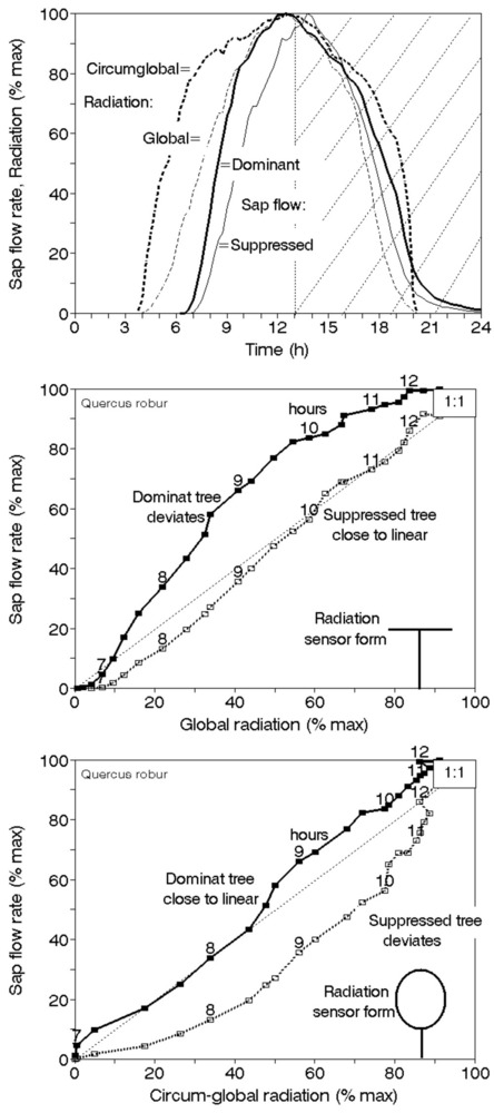
Fig. 49 - An example of mature coniferous (mostly Picea abies with admixture of other species) and pure broadleaved (Fagus sylvatica) parts of stands with contrasting optical (and most probably also similar aerodynamic) roughness (upper panel). The upper parts of tree crowns are rather smooth in Fagus, but rough in Picea. Quantitative data characterizing other similar forests stands, particularly floodplain forest (mostly Quercus robur and Fraxinus excelsior) and Norway spruce plantations are shown below (lower panel). Total leaf area as well as sunlit leaf area indexes are lower in a rather “smooth” broadleaf forest, with smaller side illumination, but substantially larger in a more “rough” coniferous forest, where light can penetrate deeper between more conical and narrower crowns.
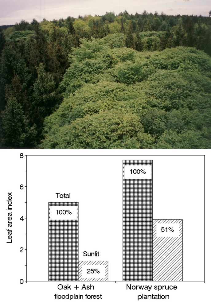
Crown water-holding capacity
Leafed crowns are important for photosynthesis and transpiration; they also provide hydrology due to their water-holding capacity, i.e., water remains in crowns after rains (Fig. 50, upper panel) and eventually falls down on soil after evaporation of part of that water. We should consider not only the rainy period but also the period after rains when water evaporation from wet surfaces is limited by high air humidity, fog, etc. We can estimate the amount of such water by comparing the relationship between daily total transpiration (or sap flow) and potential evapotranspiration during non-rainy days and days with rain or just after rains (Fig. 50, lower panel - [54]). The actual value of tree crown water-holding capacity is apparent as the difference in transpiration on rainy and non rainy days.
Fig. 50 - Droplets of water holding onto leaves and branches after rain or fog (upper panel). Water holding capacity of the whole Norway spruce tree crown estimated from the relationship between daily totals of potential evapotranspiration and tree transpiration (sap flow) measured during rainy days (and days when foliage remained wet ) and fine days (arrows show the water holding capacity of the experimental tree (about 8 dm3, i.e., over 1 mm - lower panel).
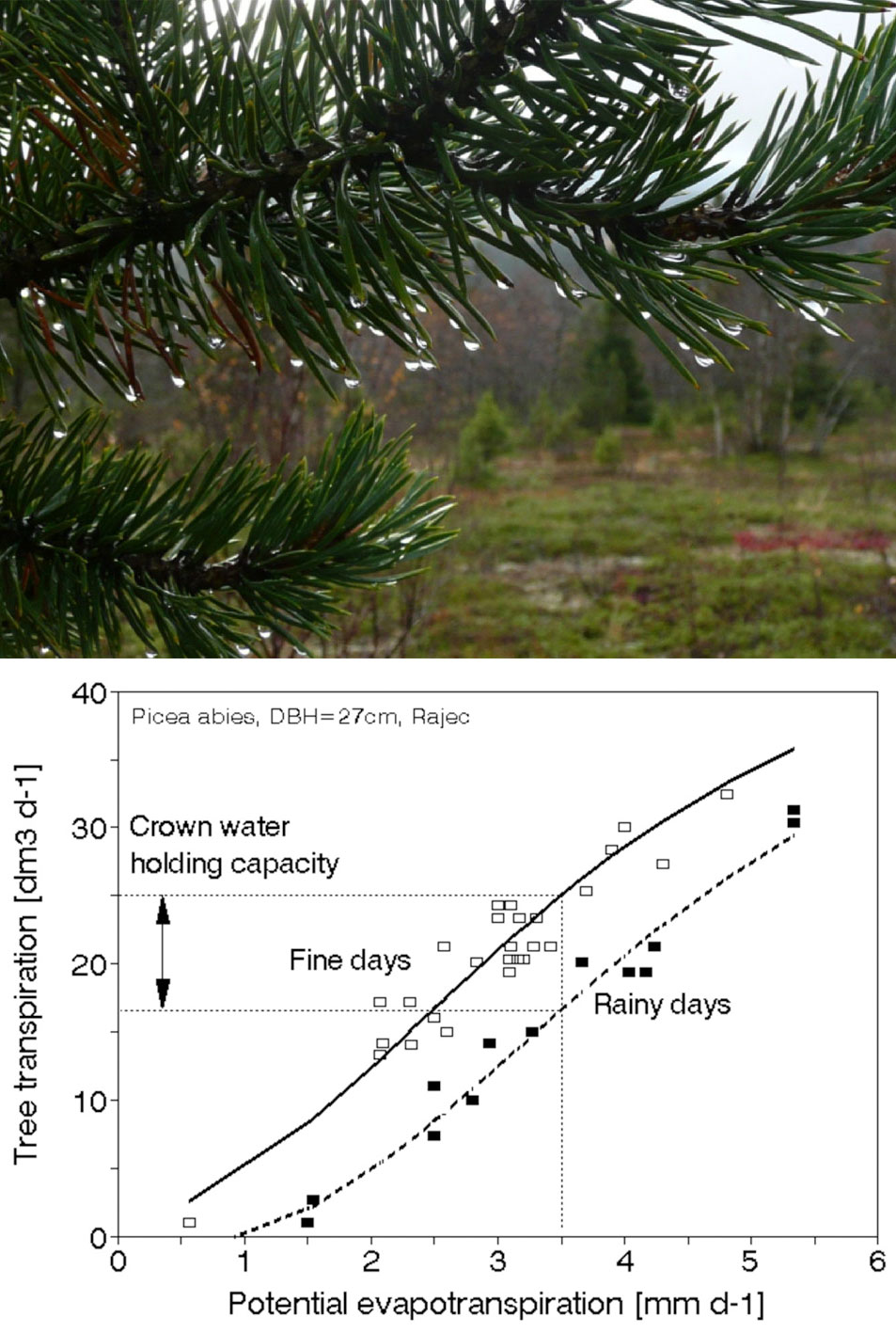
Functional parameters of tree stems [15]
Sap flow vectors in stems related to roots
Sap flow density [g cm-2 h-1] varies across tree trunks in the radial as well as circumferential direction. This can be visualized by obtaining 3D images of sap flow across sapwood using the HFD method ([163], [172]) and from data measured by multipoint sensors ([30] - see Fig. 25, Fig. 26). Flow density can be interpreted from the viewpoint of root water supply if sensors are situated at the trunk base or from the viewpoint of water loss by transpiration in different parts of the crown when measuring sap flow, e.g., at the crown base (Fig. 51, upper panel). A series of experiments based on severing different individual roots or irrigating them locally ([57], [58], [164], [169], [35]) indicated that sap flow passing through the outer sapwood layers comes mostly from superficial roots situated in shallow soil layers and that sap flow passing through the inner sapwood layers comes mostly from sinker and tap roots and deep soil layers ([156] - Fig. 51, middle panel). Because the method permits automatic recording over a broad range of time intervals (e.g., 3 s to 1 or more days), we can temporarily follow root water supply or loss in great detail and thereby analyze the functioning of the whole conducting system. This is illustrated by the record of sap flow density [g cm-2 h-1] taken at 12 measured points along the trunk radius, which forms a slightly asymmetrical curve. This curve is first converted to sap flow per individual annulus by multiplying the density values by the corresponding area of the annuli [g h-1]; then, the 2 peaks of the curve were identified and separated using the method of Novák ([177]), which is usually applied in gas chromatography. The peaks characterize flow rates from different roots (superficial and sinker) and naturally overlap when this reflects the real situation in soil ([167], [67]). The distribution of active roots situated at different depths around the stems can be estimated (Fig. 51, lower panel). This pattern can change significantly with changes in the soil water supply. Sap flow from superficial roots (indicated by the outer peak) usually decreases dramatically during drought, while the inner peak may remain the same or even temporary increase under such conditions.
Fig. 51 - Scheme for evaluation of radial patters of sap flow in stems in terms of estimation of water fractions coming from different soil depths to different parts of crown (modified from [36] - upper panel). The flow in outer layers corresponds to water supply by superficial roots (80 % of total) and the flow in inner layers corresponds to sinker roots (20 %, middle panel). Sap flow around the tree stems and in different root depths, gives its 3D distribution (lower panel), which can sometimes explain seemingly strange behavior of trees.
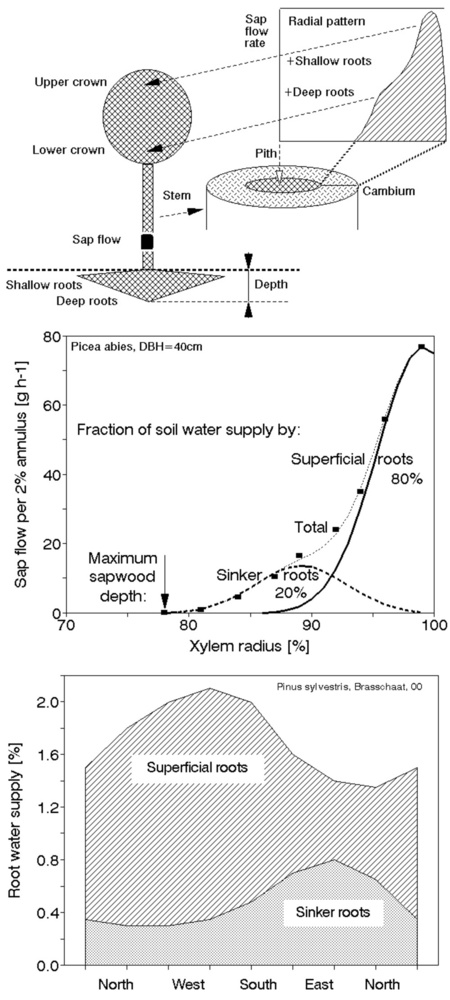
Conducting system effectiveness, tree functional stability and safety
The efficiency of the conductive system can be evaluated by comparing the theoretical conductivities (based on the Hagen-Poiseuille equation for capillaries) with the maximum seasonal transpiration (via sap flow) of the main stems and leaves (or petioles). The theoretical values have been calculated on the basis of anatomical analysis and measured differences in integrated soil and leaf water potentials. This type of study is technically demanding (it requires the application of field methods as well as microscopic methods) but useful. Two species from contrasting sites were considered: approximately 100-year-old Quercus robur trees in southernmost Moravia ([45], [47], [128] - Fig. 52, upper panel) and approximately 40-year-old Laurus azorica trees in the Canary Islands (Fig. 52, middle panel). We combined studies on: (1) stand stocking density and structure ([150]); (2) leaf distribution ([151]); (3) anatomy of stems and petioles ([153]); (4) water potential distribution ([152]); (5) annual measurement of sap flow ([107]); and finally (6) hydraulic calculation and conducting system efficiency estimates ([61]). We observed that in both species, the outermost part of the stem (very shallow in oak and rather deep in laurel) is the most important part of the tree for conducting water. The maximum measured transpiration (sap flow rate) for the stand was almost identical (95%) to the theoretical rate calculated based on petiole anatomy, but it was, on average, approximately 41 ± 1 times lower than that calculated based on stem anatomy (Fig. 52, lower panel). This illustrates the safety features of stem wood, which, due to its high vessel density, is capable of transporting all the water required even when only a small area of its vessels is functioning. In the petioles, xylem is more efficiently used, but almost all vessels must work to supply sufficient water to leaves, and any disturbance may cause leaf loss. This also explains a dangerous situation for arborists: a tree crown can be fully developed with no visible defoliation, at least over short periods of time, but this foliage could be supplied by only perhaps 5% of the well working vessels of the conductive system; the rest of the stem could be rotten, posing a great threat to the public. This feature may also affect the evaluation of the stem growth rate (e.g., annual increments over the past year or several years). A fully developed crown can supply enough assimilates for good stem growth, but this may be dependent on a single root only. If this root is damaged by chronic illness (e.g., fungal infection) or accidentally destroyed, the whole crown can decline dramatically, and stem growth can cease as well. In both cases, the application of only a visual approach could be highly misleading; verification should always be performed, ideally by applying 2 independent instrumental methods.
Fig. 52 - Stands of contrasting species (Quercus robur and Laurus azorica) growing in very different and distant sites: floodplain forest in southern Moravia (Czech Republic - upper panel) and sub-mountain forest on volcanic soil in Tenerife (Canary Islands - middle panel), respectively. Calculated theoretical sap flow (based on analysis of tree and leaf distribution in the stand plus stem and petiole anatomy) and maximum measured seasonal sap flow in the same species. When taking theoretical sap flow in petioles as 100 %, theoretical flow in stems was on average 40 and 42 x higher, respectively, but the maximum measured sap flow reached 96 and 94 % only (lower panel).
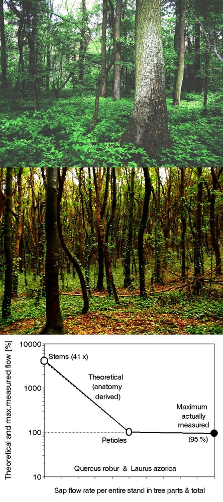
Functional parameters of root systems [16]
Root system distribution via sap flow patterns - examples of applications
Root systems growing in soils, develop under much more heterogeneous conditions than crowns; therefore, root systems vary substantially more than crowns. Sometimes this variation is not pronounced or important (although differences in tens of percentage points may play a decisive role), but in other cases, root system variation may be critical. We present several examples to illustrate different patterns of root adjustment measured using 3D sap flow distribution in stems (altogether, 700 sap flow measuring points were applied in pine - Fig. 53).
Fig. 53 - Examples of fractions of effective water absorptive tree roots estimated on the basis of sap flow radial pattern measurements. (1) Two groups of Scots pine trees growing a short distance of each other, differed in total sap flow rate and stem growth (top panel). This likely occurred because there was a sandy soil layer above the clay subsoil, 1 m deep in “shallow” soil and 4 m deep in “deep” soil, which was reflected by different fractions of root water supply. (2) A fraction of root water supplies by superficial and sinker roots in leaning trees. Trees were leaning to the West due to prevailing winds (second panel). Superficial roots were developed more in the windward direction and sinker roots were developed more in the leeward direction, all with corresponding transition zones. (3) The third panel shows the effective water absorptive root distribution in opposite stem sides of Norway spruce each of which was facing neighboring tree groups of different stocking density (see fractions of supplied water from: sparse and dense surrounding - third panel; orig). (4) Absorptive spruce root distribution growing uphill and downhill. There is highly prevailing sap flow rate from superficial roots and little flow from small sinker roots in the uphill direction, but substantially higher sap flow rate from well developed sinker roots downhill (fourth panel - orig.).
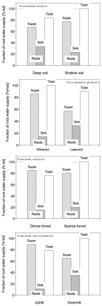
(1) Rather small but important differences in the distribution of shallow and deep roots were observed in groups of Scots pine trees growing close to each other (~50 to 70 m) in sandy soil at different depths of clay subsoil (1 and 4 m). Deep roots were almost 50% more developed in deeper soil. The sap flow rate as well as the stem growth rate was approximately 20% higher in trees growing in shallower soil (i.e., trees growing closer to the level of underground water - Fig. 53, top panel - [167]).
(2) Another example based on a larger set of trees characterizes Scots pine trees at a particular stand (the same set of sap flow sensors used above were applied). These trees were growing under the impact of frequent western winds and were leaning for about 10 deg. They developed more superficial roots in the windward direction and more sinker roots in the leeward direction (Fig. 53, second panel - modified according to [69]).
(3) Root distribution can also be adjusted gradually to different stocking densities. This became clear when measuring sap flow around Norway spruce trees that faced on one side the denser part and on the other side the sparser part of the neighboring forest. Although the difference in stocking density was approximately only 15%, root water supply and stem growth differed by approximately 30 %; roots were also 40% deeper in these trees (Fig. 53, third panel - modified according to [2]).
(4) Even larger differences between stem sides were observed in Norway spruce trees growing on steep slopes Down-slope growing roots were 3 times more developed than those growing up-slope (Fig. 53, fourth panel). These examples do not indicate that the above-described root distribution will always occur; the important message is that the available methods can be applied for getting objective data in similar studies. Application of similar methods and providing sometimes non-traditional results (such as e.g., RAI, RAI/LAI, CAI/(RAI/LAI) and many other relations is a fundamental step towards higher quality management of forest stands, modeling, etc.
Absorptive root area - via the modified earth impedance method
One of the fundamental parameters of trees is the active ion absorptive root area, a parameter that is comparable to leaf area (or preferably, to sunlit leaf area). The absorptive root area can be measured using the modified earth impedance method, which was developed for this purpose ([214], [8]). The corresponding instrumentation consists of 3-4 series of stainless steel electrodes inserted in the stem and in soil at a distance (perhaps 6-12 m) from stems and a moving electrode between the stem and the soil (Fig. 54, upper panel). The electrical conductivity of plants is based mainly on the presence of atomic ions in water. Plants can be ranked as heterogeneous electrical conductors of the second-class or heterogeneous water electrolytes. If a plant becomes part of an electric circuit (Fig. 54, middle panel), the principle of current continuity is in operation. A living, healthy and undamaged plant is a relatively poor conductor of electric current. A group of cells, e.g., wood, represents a system of resistance barriers (intercellular spaces filled with water); the electrical conductivity of such a system is omni-directional. However, there is conductance anisotropy in the system. The modified earth impedance method measures effective absorptive root area in sections with a width of 60° (of a total of 360°). Even in complex mixed forests, the system “senses” only sample trees in which electrodes are inserted. An exception is the impact of eventual anastomosis, which may simulate higher absorptive root area than would correspond to DBH. This method was tested in 12 woody species with a range of diameters (0.5 to 55 cm - [64]; and 0.5 to 120 cm, [38]) and applied in practically oriented studies ([23], [206]). It can also be modified by the application of electrical impedance spectroscopy ([193], [194], [28], [29]). The measured values for a series of sample trees representing individual DBH classes (Fig. 54, lower panel) can be converted to stand level (root area index - RAI) by calculating the DBH - root area relationships as for the case of sap flow (see Fig. 31), i.e., by deriving the values of the mean root areas, multiplying them by the corresponding number of trees and summarizing them.
Fig. 54 - Fieldwork when measuring active ion absorptive root area using a series of current electrodes at the tree trunk and in the soil at a distance (corresponding to the 60 deg section) and potential electrodes at the tree base along with a movable electrode, and corresponding cables (upper panel). Below, the scheme of measurement with the modified earth impedance method using a logometer (earth/ ground tester Fluke - middle panel) is depicted. An example of the active tree root absorptive area in Norway spruce (Picea abies) includes trees of different ages (40 to 100 years) grown at sites at different distances (lower panel).
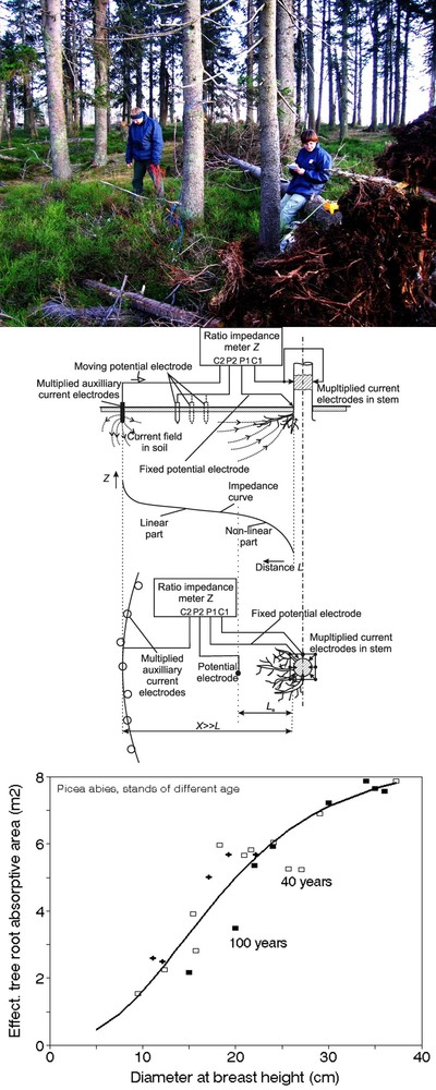
Examples of the application of active absorptive root system area in trees
Two operators can measure the actual absorptive area of tree root systems rather quickly, e.g., in approximately 2-3 hours, by using the modified earth impedance method on sections oriented according to their azimuths and on whole trees. Reasonably large sets of trees can be characterized in this way, which facilitates the practical application of results. Two examples can be provided. (1) Spruce trees (Picea sitchensis) were grown in rows with different spacing and in soil of different moisture in Scotland ([23], [38]). Mea-surements demonstrated that the actual absorptive root area was, on average, approximately 50% larger along rows than across (this corresponded to the distribution of coarse roots on wind-fallen trees: these always felled across, never along rows). The contrasting root distribution increased with increasing soil moisture (Fig. 55, upper 2 panels). (2) Large oak trees (Quercus robur) were found growing on a lawn strip along the road (between a road with a parking lot and a brick fence with a loamy walking pavement along it) in the southern Czech Republic. Fungi damaged some of these trees; younger trees (200 years old) exhibited little or no damage, while older trees (up to 400 years old) were usually seriously damaged, but the type of damage was different. The issue concerned which trees represented a dangerous threat to the public and which trees could be considered safe for a longer period of time ([206]). The extent of rotten parts of stems (measured by the acoustic method) as well as of roots (using the modified impedance method) plays a role here. The results showed that roots were always damaged in the direction across the road and that the most severe root damage corresponded to the most severe stem damage (completely rotten and opened stems). This kind of damage always occurred only in the same direction as the fence/pavement (Fig. 55, lower 2 panels). Strong hypoxia in the compacted soil below the pavement was again the main factor in tree decline.
Fig. 55 - Examples of active absorptive root area measurements (columns represent mean values and thick lines standard errors) applied for estimation of Sitka spruce root distribution across and along rows (picture and figure in upper two panels) and Pedunculate oak root distribution in trees growing along roads, where they were damaged from the road side during road building and from the opposite side (to the fence) by unfavorable soil conditions (lower two panels). Soils were rather wet in both cases, but wet in “trenches” on both sides of each spruce row and in places with high compression and increased anti-ice salt content under pavement along the fence in oak.
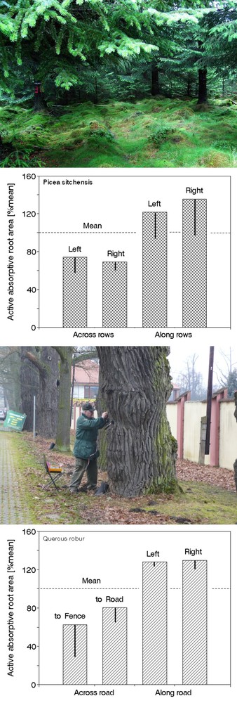
The estimation of RAI (i.e., absorptive RAI, RAIabs) permits a comparison with LAI (or preferably, sunlit LAI, LAIsun) and therefore an evaluation of the RAIabs/LAIsun ratio, which can be understood as a structural tree balance (Fig. 56, upper panel). This is a very important parameter (it is much more often applied, e.g., in agriculture) that often indicates the probability of tree survival under unfavorable environmental conditions. This can be demonstrated by comparing several Norway spruce stands with different soil water regimes and stand densities ([36], [37] - Fig. 56, lower panel). Similar, but still modified information represents, e.g., cambium area index related ratio, CAI/( RAIabs/LAIsun), etc.
Fig. 56 - The tree structural balance demonstrated on this beech sapling (upper panel) is shown with comparison of values of leaf area index, and the balance is expressed as the root/leaf area ratio in Norway spruce stands growing on loamy soils and peat land suffering severe drought (lower panel). Sparse forest edge has low leaf area index, while both dense forest keep it high. The ratio of root/leaf area indices is OK when it reaches values roughly between 4 and 9 % for dense and sparse forest, but when it reaches around 2 % only, which may be enough when the peat is well watered, but became deadly critical under drought.
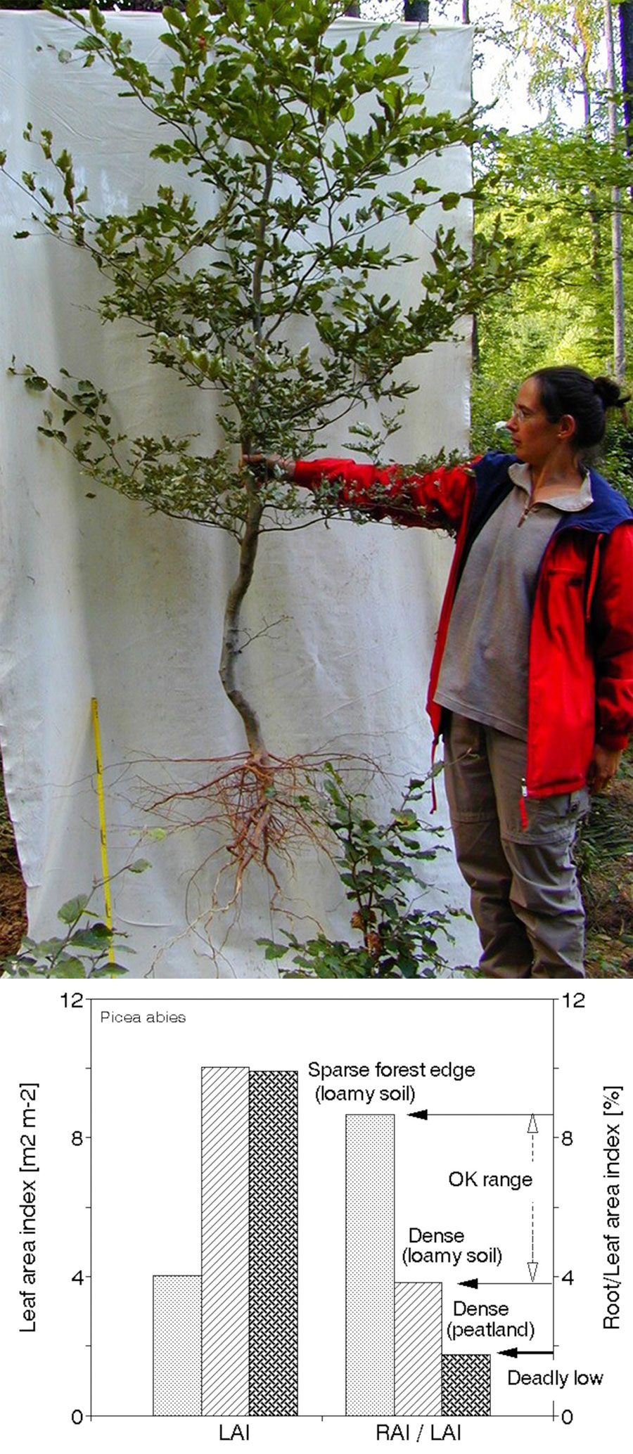
Resinous systems and pressure in tissues
In coniferous trees, resistance to pests is, to a large extent, based on the functioning of the resin system. Oleoresin (a rich mixture of terpenes of different boiling points, roughly 70 to 200 °C) is created within the epithelium parenchymatic cells of resin ducts situated in the sapwood and phloem. These ducts create a dense network in the vertical and radial directions; the density of vertical ducts (0.09 mm in diameter) is approximately 60 per square centimeter of sapwood cross-section in Scots pine, although only ducts in the 10-15 outer annual rings are functional. The density of radial ducts (0.03 mm in diameter) situated in pith rays, through which flow assimilates from the phloem, is almost twice as large. The resin content of wood is approximately 7% of its dry mass (Fig. 57, upper panel - [103], [146]). Liquid resin is toxic and, if the cells are sufficiently supplied with sugars and water, is kept under high positive pressure (10 to 15 bars) due to the osmotic force of the cells, if they are sufficiently supplied by assimilates (to produce terpenes) and water (to have turgor). Under such conditions, water is sucked out of neighboring tracheids when xylem water potential of tracheids becomes lower than that of the epithelium cells, the gradient of water potential is reversed, and water is sucked out of the epithelium cells, causing an immediate decrease in pressure (Fig. 57, lower panel - [143]). Under these conditions, the defensive system ceases to function; no oleoresin is released, and tissues can be easily attacked
Fig. 57 - Resinous system of coniferous trees and its relation to water regime and primary attraction for bark beetles. Cross section of xylem shows position of the resin duct surrounded by tracheids (upper panel). Diurnal courses of sap flow in trees, pressure changes in the resinous system (resin ducts) and water potential changes in tracheids (lower panel). The positive pressure of resin goes in parallel with tissue water potential, but on the positive part of pressure scale. However it can also move to negative values, when water potential in tracheids is very low under drought (here visible around noon). Resinous system is then loosing defensive properties of course and allowing easy bark beetle attack (modified from [143]).
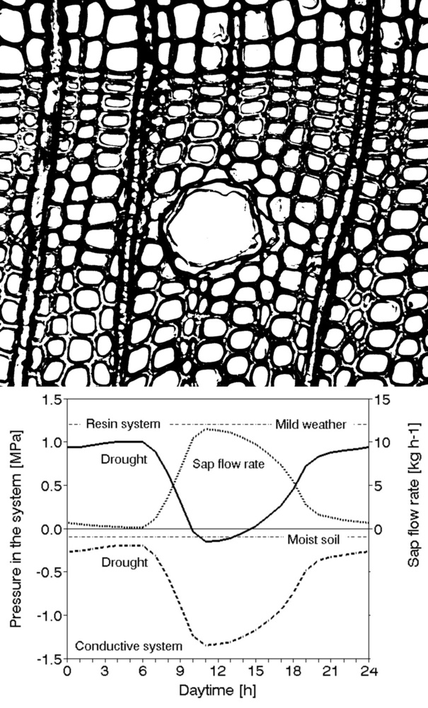
Root system distribution, sap flow and tree bark beetle attack
Trees with deep roots usually occupy large volumes of soil and therefore have a large amount of soil water storage at their disposal. This makes them physiologically more stable and more resistant to biotic pests (fungi or insects). The considerations described in the previous section emphasize the importance of tree water relations and rooting depth for tree survival ([1]). Trees growing in extremely shallow (5 to 10 cm) soil, e.g., on flat rocks or peat, are unable to develop any sinker roots (Fig. 58, upper panel), while trees growing in deeper soil, at least in places, e.g., between stones or rocks, can develop several sinker roots (Fig. 58, middle panel). The bark beetle attacked less transpiring trees with no sinker roots, while intensively transpiring trees with at least some developed sinker roots (which were able to redistribute periodically water from deeper to shallow soil layers via superficial roots) were more resistant (modified from [1] - Fig. 58, lower panel). Because the fraction of superficial and sinker roots can be rather easily determined by sap flow vector analysis, it is also possible to assess which trees are particularly at risk primarily to drought and secondarily to bark beetle under given site conditions.
Fig. 58 - Root distribution in Norway spruce (Picea abies) trees associated with bark beetle attack in neighboring trees of similar size and crown form and leaf density. The very shallow root system (only superficial roots were developed - upper panel) and deeper root system (with developed at least some sinker roots ) are shown in the middle panel. Effective absorptive root distribution estimated via radial sap flow patterns is shown in the lower panel. The fraction of root water supply from superficial and sinker roots (in % of total) - left scale and total root water supply - right scale.
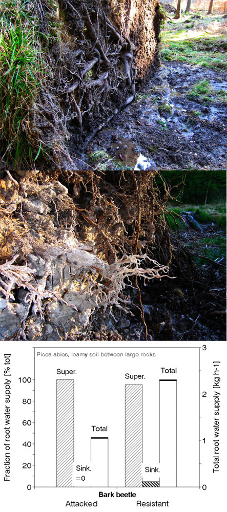
Volatile substances in air (“tree smells”) and their information value
In addition to the “visible world of trees,” trees also create an “invisible world”; by this, we mean “smells” (mostly volatile terpenes) that are emanated into the atmosphere as well as other substances that trees, like all plant species, release into soils. Liquid resin present in different tissues have different composition over short distance, e.g., in resin blisters on seeds (Fig. 59), resin cavities in bark, resin ducts at individual annual rings, etc. The contents of these compounds differed between tissues and within the same tissue when assayed at larger distances or in parts of the tree separated by anatomical barriers. Substances released into soils are active only over relatively short distances (probably not much beyond the reach of root systems), but volatile compounds can spread due to their high diffusion coefficients and can be moved by wind over long distances. The ability to spread underlies their important role as information media. Tree smells are usually composed by many volatile substances: primarily hemiterpenes in broadleaf trees (which we cannot naturally detect well), monoterpene hydrocarbons (ranging from santene and α-pinene to limonene), as well as substances with higher boiling points and molecular weights (sesquiterpenes, terpene alcohols such as borneol, terpineol and others) up to almost nonvolatile diterpenes (rosin - [244], [245]). These substances and their concentrations can provide important information about tree species and their state of health as well as information to other organisms, especially insects. The volatile fraction of oleoresin can be released when tissues are even slightly mechanically damaged (e.g., by shrinking during drought - [39], [42]) and can serve as a signal, e.g., for bark beetles. Trees already weakened by drought attract insects and can then be easily killed e.g., by intensive bark beetle attack. However, by using special instrumentation (ultratrace analysis by gas chromatography), we can obtain similar information from this material and check the health state of trees this way in time. An example of the analysis of a wide spectrum of terpenes illustrates the concentration of terpenes with C4 to C10 effective carbons (in the range of ng m-3 or less) emanating from Norway spruce tissues (mostly needles) are shown here (Fig. 60, upper panel). Monoterpene hydrocarbons and terpene alcohols prevailed in this case. Other substances were found only in small amounts in otherwise clear forest air. Healthy trees produce a more-or-less homogeneous smell that changes dramatically under drought conditions. Usually, a short-term wave occurs temporarily in trees under severe drought, but the emanation rate quickly decreases and becomes much lower (Fig. 60, lower panel, modified from [44]). The odor of dry tissues is not attractive to insects; therefore, they do not attack such trees. Air analysis by ultratrace methods of gas chromatography can provide important information about species composition (trees, herbaceous plants, fungi and bacteria) and, consequently and indirectly, forest health.
Fig. 59 - Upper panel: cross-sectioned seed of Silver fir on millimeter matrix. OS = ovuliferous scale; Br = bractea; W = wing; m = median plane; e = embryo; en = endosperm. Individual resin cavities (visible on the seed surface like blisters and marked A, B, D, E) appear with regard to their adaxial (ad) or abaxial (ab) locations and medial (med) or marginal (marg) seed side. Lower panel: the content of individual monoterpene hydrocarbon mixture in the resin from various resin cavities of Abies alba seed. The center of rectangels designates the mean value of the terpene content in the resin. of a single cavity (calculated as percentage of the mean from all resin cavities, % of X). Horizontal sides of rectangles designate the limits of confidence interval for P0.05. Individual resin cavities are designated according to their position (abaxial-adaxial, medial-marginal) on the seed (see the upper panel), according to [44]).
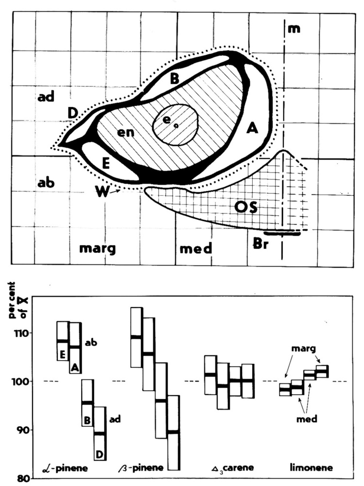
Fig. 60 - Air concentration of volatile terpenes (in the range of C4 to C10 of effective carbons, i.e., approx. isoprene to monoterpenes) as estimated by the gas chromatography. This represents a “normal smell” of spruce branches (such smells partially differ in different tissues and their positions in trees - upper panel). Emanation rate of terpenes from spruce, which can serve as primary attractants for bark beetles, especially when tissues are damaged e.g., by drought and emanation rate temporarily increases or modifies. The emanation rate is higher when a tree is healthy, but decreases significantly in dry tissues, when most terpenes have already vaporized from the bark or needle surface (lower panel). The smell of dry tissues is not interesting for bark beetles; therefore they do not attack such trees any more (modified from [52]).
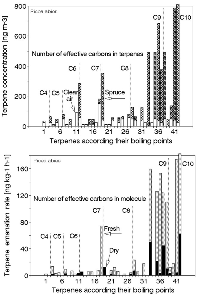
Conclusions [17]
The above-described methods objectify and provide additional information to classical forest biometric methods, which is important especially in cases, when these methods themselves are not sufficient to explain some observed situations. They can contribute with packages of non-traditional data sets e.g., to the evaluation of direct and indirect impacts of global climatic changes, improving our understanding of processes that occur in differentiated natural environments and evaluation of stability of forest ecosystems. Some illustrative examples have been provided.
In this presentation, details were avoided, thereby allowing the text to be substantially shortened (to approximately one paragraph per method); for these details, please see the cited literature sources. We tried to minimize the addition of detail explanations, for this reason we better applied more illustrating figures and pictures (completely avoiding presentation of actual data), because the information is more compressed in illustrations and the number of pages gets smaller this way. We included literature sources for each method or each paragraph anywhere possible, so a reader who wants to get more information, has these sources available.
Usually, institutions for forest management etc. inform their management practices based on valuable annual and season stem growth data measured on a large scale (usually nationally). The data provide crucial information about timber production and yield. Plenty of literature is available in this scientific field. Therefore, we mostly avoided this kind of research, focusing on other features, which are not so well known. This is the principle of Precision Forestry: utilization of a better quantitative understanding of hydrological and ecological processes and facts that are needed for correct decision making.
We can expect that this tendency will continue and that ground-based measurement will be still more intensively connected with remote sensing systems. This will provide a possibility to use ground-based data for calibration of complex spectra obtained by specialized cameras for better coverage of large areas and therefore faster practical application of the obtained knowledge.
Acknowledgements
The study was done within the framework of the project of Internal agency of the Faculty of Forestry and Wood Technology No.73/2013: “Ecophysiological behavior of Norway spruce (Picea abies (L.) Karst.) in forest typological and geobiocenological units of highlands” (Dept. of Forest Botany, Dendrology and Geobiocenology) and VZ MSM 6215648902 “Forest management strategy in regions with special status of protection” (Dept. of Forest Management). The work was also partially supported by OP Education for Competitiveness (European Social Fund and the state budget of Czech Republic) CZ.1.07/2.3.00/30.0017 Postdocs in Biological Sciences at MENDELU. The authors are obliged to Dr. Jan Štykar and Dr. Antonin Kusbach for their valuable comments to the manuscript and to Dr. Zdenka Podhajská for her help with editing. They are also obliged to Prof. Radomír Ulrich and Ing. Tomas Veverka (all from the Faculty of Forestry and Wood Technology) for their help with air-spade excavation of root systems.
References
Gscholar
Gscholar
Gscholar
Gscholar
Gscholar
Gscholar
Gscholar
Gscholar
Gscholar
Gscholar
Gscholar
Gscholar
Gscholar
Gscholar
Gscholar
Gscholar
Gscholar
Gscholar
Gscholar
Gscholar
Gscholar
Gscholar
Gscholar
CrossRef | Gscholar
Gscholar
Gscholar
Gscholar
Gscholar
Gscholar
Gscholar
Gscholar
Gscholar
Gscholar
Gscholar
Gscholar
Gscholar
Gscholar
Gscholar
Gscholar
Gscholar
Gscholar
Gscholar
Gscholar
Gscholar
Gscholar
Gscholar
Gscholar
Gscholar
Gscholar
Gscholar
Gscholar
Gscholar
Gscholar
Gscholar
Gscholar
Gscholar
Gscholar
Gscholar
Gscholar
Gscholar
Gscholar
Gscholar
Gscholar
Gscholar
Gscholar
Gscholar
Gscholar
Gscholar
Gscholar
Gscholar
Gscholar
Gscholar
Gscholar
Gscholar
Gscholar
Gscholar
Gscholar
Gscholar
CrossRef | Gscholar
Gscholar
Gscholar
Gscholar
Gscholar
Gscholar
Gscholar
Gscholar
Gscholar
Gscholar
Gscholar
Gscholar
Gscholar
Gscholar
Gscholar
Gscholar
Gscholar
Gscholar
Gscholar
Gscholar
Gscholar
Gscholar
Gscholar
Gscholar
Gscholar
Gscholar
CrossRef | Gscholar
CrossRef | Gscholar
Gscholar
Gscholar
Gscholar
Gscholar
Gscholar
CrossRef | Gscholar
Gscholar
Gscholar
Gscholar
Gscholar
Gscholar
Gscholar
Gscholar
Gscholar
Gscholar
Gscholar
Gscholar
Gscholar
Gscholar
Gscholar
Gscholar
Gscholar
Gscholar
Gscholar
Gscholar
Gscholar
Gscholar
Gscholar
Gscholar
Gscholar
Gscholar
Gscholar
Gscholar
Gscholar
Gscholar
Gscholar
Gscholar
Gscholar
Gscholar
Gscholar
Gscholar
Gscholar
Gscholar
Gscholar
Gscholar
Gscholar
Gscholar
Gscholar
CrossRef | Gscholar
Gscholar
Gscholar
Gscholar
Footnotes
Authors’ Info
Authors’ Affiliation
Nadezhda Nadezhdina
Miroslav Trcala
Jaroslav Simon
Faculty of Forestry and Wood Technology, Mendel University in Brno, Zemedelská 3, 61300 Brno (Czech Republic)
Corresponding author
Paper Info
Citation
Cermák J, Nadezhdina N, Trcala M, Simon J (2015). Open field-applicable instrumental methods for structural and functional assessment of whole trees and stands. iForest 8: 226-278. - doi: 10.3832/ifor1116-008
Academic Editor
Marco Borghetti
Paper history
Received: Aug 31, 2013
Accepted: May 13, 2014
First online: Sep 03, 2014
Publication Date: Jun 01, 2015
Publication Time: 3.77 months
Copyright Information
© SISEF - The Italian Society of Silviculture and Forest Ecology 2015
Open Access
This article is distributed under the terms of the Creative Commons Attribution-Non Commercial 4.0 International (https://creativecommons.org/licenses/by-nc/4.0/), which permits unrestricted use, distribution, and reproduction in any medium, provided you give appropriate credit to the original author(s) and the source, provide a link to the Creative Commons license, and indicate if changes were made.

Web Metrics
Breakdown by View Type
Article Usage
Total Article Views: 73518
(from publication date up to now)
Breakdown by View Type
HTML Page Views: 60575
Abstract Page Views: 4700
PDF Downloads: 6539
Citation/Reference Downloads: 83
XML Downloads: 1621
Web Metrics
Days since publication: 4271
Overall contacts: 73518
Avg. contacts per week: 120.49
Article Citations
Article citations are based on data periodically collected from the Clarivate Web of Science web site
(last update: Mar 2025)
Total number of cites (since 2015): 17
Average cites per year: 1.55
Publication Metrics
by Dimensions ©
Articles citing this article
List of the papers citing this article based on CrossRef Cited-by.
Related Contents
iForest Similar Articles
Research Articles
Links between phenology and ecophysiology in a European beech forest
vol. 8, pp. 438-447 (online: 15 December 2014)
Research Articles
Electrochemical in-situ studies of solar mediated oxygen transport and turnover dynamics in a tree trunk of Tilia cordata
vol. 10, pp. 355-361 (online: 07 March 2017)
Research Articles
Relationship between volatile organic compounds released and growth of Cunninghamia lanceolata roots under low-phosphorus conditions
vol. 11, pp. 713-720 (online: 06 November 2018)
Research Articles
Allometric relationships for predicting the stem volume in a Dalbergia sissoo Roxb. plantation in Bangladesh
vol. 3, pp. 153-158 (online: 15 November 2010)
Research Articles
Evaluation of fast growing tree water use under different soil moisture regimes using wick lysimeters
vol. 6, pp. 190-200 (online: 08 May 2013)
Research Articles
Energy production of poplar clones and their energy use efficiency
vol. 7, pp. 150-155 (online: 23 January 2014)
Research Articles
Extreme climatic events, biotic interactions and species-specific responses drive tree crown defoliation and mortality in Italian forests
vol. 17, pp. 300-308 (online: 30 September 2024)
Research Articles
Effect of family, crown position, number of winter buds, fresh weight and the length of needle on rooting ability of Pinus thunbergii Parl. cuttings
vol. 9, pp. 370-374 (online: 11 January 2016)
Research Articles
Estimation of stand crown cover using a generalized crown diameter model: application for the analysis of Portuguese cork oak stands stocking evolution
vol. 9, pp. 437-444 (online: 02 December 2015)
Research Articles
Methods to inventory and strip thin in dense stands of aspen root suckers
vol. 8, pp. 590-595 (online: 22 April 2015)
iForest Database Search
Google Scholar Search
Citing Articles
Search By Author
Search By Keywords
PubMed Search
Search By Author
Search By Keyword


