Modeling stand mortality using Poisson mixture models with mixed-effects
iForest - Biogeosciences and Forestry, Volume 8, Issue 3, Pages 333-338 (2015)
doi: https://doi.org/10.3832/ifor1022-008
Published: Sep 05, 2014 - Copyright © 2015 SISEF
Research Articles
Abstract
Stand mortality models play an important role in simulating stand dynamic processes. Periodic stand mortality data from permanent plots tend to be dispersed, and frequently contain an excess of zero counts. Such data have commonly been analyzed using the Poisson distribution and Poisson mixture models, such as the zero-inflated Poisson model (ZIP), and the Hurdle Poisson model (HP). Based on mortality data obtained from sixty Chinese pine (Pinus tabulaeformis) permanent plots near Beijing, we added the random-effects to the Poisson mixture models. Results showed that the random-effects in the ZIP model was not convergent, and HP mixed-effects model performed better in modeling stand mortality than the Poisson fixed-effects model, the Poisson mixed-effects model, the ZIP fixed-effects model and the HP fixed-effects model. Moreover, the HP model accounts for two sources of dispersion, the first accounting for extra zeros and the second accounting to some extent for the dispersion due by individual heterogeneity in the positive set. We also found that stand mortality was negatively related to stand arithmetic mean diameter and positively related to dominant height.
Keywords
Hurdle Model, Mixed Model, Poisson Model, Stand Mortality, Zero Inflated Model
Introduction
An important component equation of whole stand models is one that predicts, explicitly or implicitly, stand mortality (trees ha-1) over a period of time ([31]). However, in contrast to other stand variables, it is often difficult to accurately describe patterns of mortality across stand and site conditions ([16]). This may be because tree mortality is a complex process affected by environmental, pathological, and physiological factors ([32]). Due to the uncertainty of the tree mortality process, mortality remains one of the least understood components of natural stand growth processes ([2]). Over the years, researches have focused on individual tree mortality for analyzing stand mortality: tree mortality was predicted with a logistic model ([34]), and aggregated for estimating stand mortality. Unfortunately, collecting detailed tree information to develop a tree mortality model is costly ([23]). What is more, stand mortality predicted from a tree mortality model often suffers from an accumulation of errors and subsequently poor accuracy and precision ([25], [34]). Woollons ([31]) used a two-step method to estimate the stand mortality. However, this method does not admit a well-defined stochastic structure that can serve as a basis for inference ([1], [35]).
Mortality is a complicated stochastic process influenced by several stand characteristics and environment factors, which often exist with complex interactions. It is hardly possible to capture all of the observed variability in empirical mortality data. The evolution of the mixed-effects modeling methodology provided a statistical method capable of explicit modeling stochastic structure is a possible approach for solving this problem ([4]).
In addition, it has to be considered that a relatively high number of permanent sample plots has no occurrence of mortality, even over periods of several years. Therefore, mortality data are truncated and characteristically exhibit varying degrees of dispersion and skewness in relation to the mean. Moreover, the data often contain an excess number of zero counts. The least squares method implicitly presumes that the data are Gaussian distributed with constant variances, or at least satisfy the Gauss-Markov conditions. If the least squares method is applied to data with a large proportion of zero counts, the estimated results will be biased. Alternatively, if only nonzero mortality observations are used for model development, then mortality will be overestimated ([31], [8]). In recent years, there has been considerable interest in models for count data, such as manufacturing defects ([18]), patent applications ([6]), species abundance ([13]), medical consultations ([12]), use of recreational facilities ([27]). There are also a few studies that have addressed this issue in forestry (e.g., [1], [10], [35]).
Although many forest models accounted for mixed effects such as tree diameter growth models ([17], [28]), height growth models ([9]), and others ([11], [29]), compared with the substantial literature on cross-sectional zero-inflated count data, relatively few studies have considered mixed effects in the count-data models in forestry ([13], [26]), due to the complexity and difficulty in obtaining convergence, especially for applications in forestry ([19]). The objective of this study was to develop and compare the Poisson mixture models with and without random-effects for predicting stand mortality over a period of time.
Material and methods
Dataset
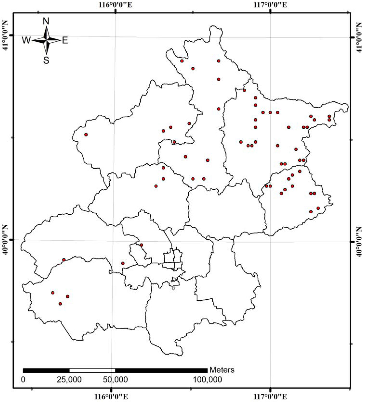
A systematic sampling of permanent, square-shaped plots (0.067 ha) was carried out by the Inventory Institute of Beijing Forestry with a 5-year re-measurement interval. Overall, sixty plots were sampled in several Chinese pine (Pinus tabulaeformis Carr.) plantations situated on upland sites of Beijing (Fig. 1): 44 plots were measured in 1986, 58 plots in 1991, and 60 plots in 1996, 2001. The final dataset consisted of measurements from 162 stands obtained between 1986 and 2001. Summary statistics of stand variables are presented in Tab. 1. The climate in the studied area is warm temperate and semi-humid. Mean annual temperature ranges from 9 to 11 °C, and rainfall varies between 500 and 700 mm.
Fig. 1 - Location of the 60 plantations of Chinese pine (Pinus tabulaeformis Carr.) studied in this investigation. The black lines on the map represent the boundaries of the Beijing’s administrative region.
Tab. 1 - Summary statistics of stand-level variables. (SD): standard deviation: (SM): stand mortality counts in a plot; (A): stand age; (H): stand dominant height; (N): stand density; (B): stand basal area; (Dm): stand arithmetic mean diameter; (Al): altitude; and (Rs): the relative spacing. The relative spacing was computed as a function of dominant height and stand density: Rs = (10000/N)0.5/H.
| Variables | Min | Max | Mean | SD |
|---|---|---|---|---|
| SM (trees plot-1) | 0 | 38 | 2.6 | 6.46 |
| A (years) | 12 | 55 | 27 | 8.46 |
| H(m) | 2.5 | 17.4 | 6.4 | 2.83 |
| N (trees ha-1) | 132 | 2164 | 933 | 492.24 |
| Dm (cm) | 5.8 | 16.13 | 9.76 | 2.4 |
| Rs (trees ha-1 m-1) | 0.17 | 3.45 | 0.71 | 0.63 |
| Alt (m) | 140 | 1400 | 449.91 | 268.09 |
Variable selection
Independent variables characterized by a meaningful biological interpretation were selected among those describing altitude (Alt), site conditions (dominant height, H) and stand characteristics (stand age, A; stand density, N; stand arithmetic mean diameter, Dm; relative spacing etc.). Multicollinearity among independent variables was verified by applying the variance inflation factor (VIF) test. According to a common rule-of-thumb, multicollinearity among variables was considered to occur when VIF > 5. In addition, variables showing p > 0.05 after a pairwise Student’s t-test were discarded from the model.
Poisson model
Count data models are a subset of discrete-response regression models aimed to describe the number of occurrences or counts of an event. Poisson regression is the simplest regression model for count data, and the probability mass function (PMF) is expressed as follows (eqn. 1):
where y refers to the random variable of stand mortality (dead counts), y = 0, 1, 2, …, n, and λ > 0. A Poisson regression model is obtained by relating the mean λ to a vector of independent variables X, by λ = exp(Xβ), where β is the vector of regression coefficients to be estimated. A characteristic of the Poisson probability function (eqn. 1) is that the mean and the variance are equal, that is Var[Y | X] = E[Y | X] = λ. When data do not fit to the Poisson distribution, it is typically because of overdispersion, i.e., the model’s variance exceeds the mean value.
ZIP model
ZIP (zero-inflated Poisson) model is a mixed model combining a Poisson distribution with a point mass at zero. In zero-inflated Poisson model, there are two sources of zeros, deriving both from the point mass and from the count component ([18]). Actually, two regression equations are created in zero-inflated Poisson models, one predicting whether the count occurs and the other predicting differences on the occurrence of the count (Poisson - [15]). ZIP is a very flexible model for handling data dispersion, and the PMF for ZIP is given by (eqn. 2):
where p is the probability of a zero count in excess, and (1-p) is the probability of belonging to the Poisson component. Logistic regression is commonly used to fit the point mass component: logit(p) = Log(p/1-p) = Xδ. As for the Poisson component, it is obtained from a vector of independent variables, λ = exp(Xβ), where X is a vector of independent variables, δ and β are vectors of the parameters to be estimated.
HP model
HP (Hurdle Poisson) model, originally proposed by Mullahy ([24]) in the econometrics field ([5]), is another model class capable of dealing with excess zero counts. However, HP is slightly different from ZIP model with all zero counts from two different sources, and assumes that zero counts might come from a single statistical process ([21]).
Similar to ZIP model, HP model is the combination of a logit regression modeling point mass at zero and a truncated Poisson regression modeling count component. Its PMF is expressed as follows (eqn. 3):
The point mass component is obtained by logistic regression using logit(p) = Log(p/1-p) = Xδ, while the Poisson component is obtained from a vector of independent variables, λ = exp(Xβ).
In this study, a plot-level random-effects parameter was added to the intercept for the Poisson model, and to the intercept of the Poisson component for the estimation of positive mortality counted for ZIP model and HP model. The random-effect parameter was defined as: u~N(0, v), where v is the variance.
All parameter vectors can be estimated through the optimization of the likelihood function, that is, by applying the maximum likelihood method (ML). The unstructured covariance structure ([20]) was used for describing the variance-covariance structure of random effects. Parameter estimation was implemented using the SAS/ STAT NLMIXED procedure.
Model selection and goodness-of-fit
Performances of the Poisson fixed-effects model, ZIP fixed-effects model, HP fixed-effects model and corresponding mixed-effect models calibrated with the same data set can be compared by using the log-likelihood values [-2L(φ,y)], the Akaike information criterion (AIC), as well as the Bayesian information criterion (BIC). Smaller values of AIC, BIC and -2L(φ,y) indicate better performances for the model considered. Both AIC and BIC rely on a penalized maximum log-likelihood value. As the penalty is based on the number of model parameters, the use of these statistics ensures the best trade-off between the goodness-of-fit and the number of parameters included in the model. The penalty is more influential in the BIC, making this criterion more conservative than the AIC ([10]).
The Vuong test is a popular method to compare two non-nested models for count data ([30]). If we define (eqn. 4):
where Pj(Yi | Xi) is the predicted probability of the observed count for the i-th case in the j-th model, then Vuong statistic to test the hypothesis E(mi=0) is expressed as follows (eqn. 5):
where n represents the number of count classes. The first model should be preferred when V>1.96, while the second should be preferred in the case of V<-1.96 ([21]).
Because of the use of maximum log-likelihoods, AIC, BIC, and Vuong parameters are relative statistics, as they do not ensure that the fit of the “best” model is good. Hence, residual plots (residual values between predicted and observed probabilities plotted against the count class j) were used to detect any predictive bias of the models and assess their goodness-of-fit ([18], [10]). The residual rj, between predicted probabilities and observed probabilities was computed as (eqn. 6):
where # represents the frequency of observations yi in the count class j, n is the number of count classes, and P(y=j) is the predicted probability that an observation belongs to the j-th count class.
Results and discussion
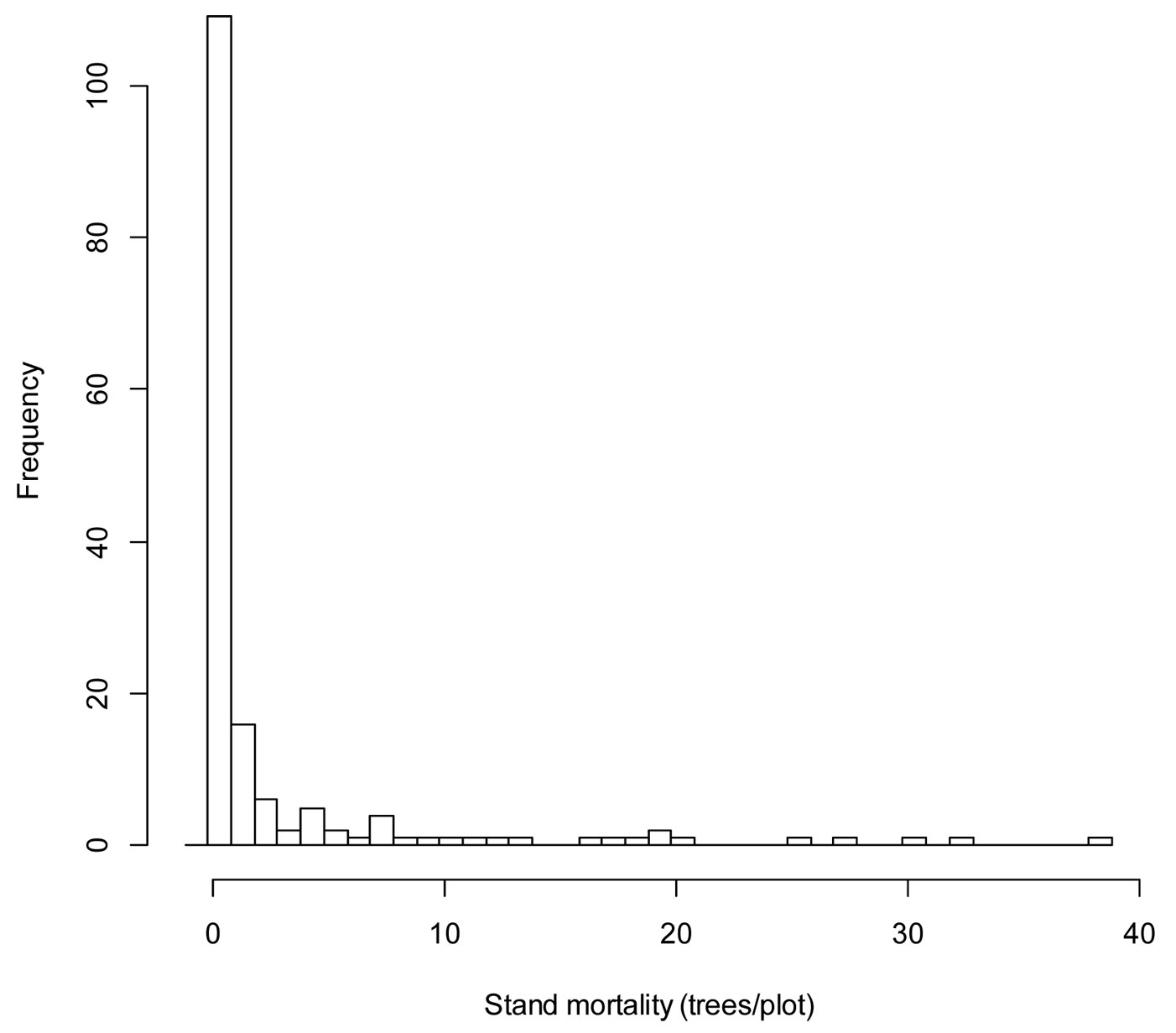
In this study, a relatively high number of the plots considered has no occurrence of mortality. Mortality data are zero-bounded and characteristically exhibit varying degrees of dispersion around the mean and skewness (Fig. 2). According to the VIF test, no multicollinearity was found among the independent variables included (VIF<5).
Fig. 2 - Histogram of stand mortality for Chinese pine obtained from the sixty plots selected in the study area.
During the processes of estimating all the six models considered, we found that the ZIP mixed-effects model was not convergent, so the following results were obtained from the remnant five models.
Results showed that the statistics -2L(φ,y), AIC and BIC obtained for the HP mixed-effects model were much smaller than those of the other models (Poisson fixed-effects model, Poisson mixed-effects model, ZIP fixed-effects model and HP fixed-effects model - Tab. 2), suggesting that the HP mixed-effects model provided the “best fit”.
Tab. 2 - Fit statistics of Poisson fixed-effects model, Poisson mixed-effects model, ZIP fixed-effects, HP fixed-effects model, and HP mixed-effects model.
| Statistic | Poisson-fixed | Poisson-mixed | ZIP-fixed | HP-fixed | HP-mixed |
|---|---|---|---|---|---|
-2L(φ,y) |
1305.8 | 658.9 | 783.1 | 783 | 513.8 |
| AIC | 1319.8 | 670.9 | 795.1 | 795 | 527.8 |
| BIC | 1341.4 | 683.8 | 813.6 | 813.6 | 542.8 |
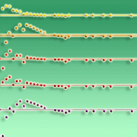
Poisson fixed-effects and Poisson mixed-effects models were found to largely underestimate the zero-class counts, while ZIP fixed-effects, HP fixed-effects and HP mixed-effects models exactly estimated the zero dead counts (Fig. 3). The residuals rj of the Poisson mixed-effects model were smaller than those obtained for the Poisson fixed-effects model, while the HP mixed-effects model showed lower residuals than those obtained from the HP fixed-effects, ZIP fixed-effects and Poisson mixed-effects model (Fig. 3).
Fig. 3 - Plots of residuals for the Poisson fixed-effects model (A), Poisson mixed-effects model (B), HP fixed-effects model (C), HP mixed-effects model (D), and ZIP fixed-effects model (E). (rj): residuals between predicted and observed probability as computed by using the eqn. 6.
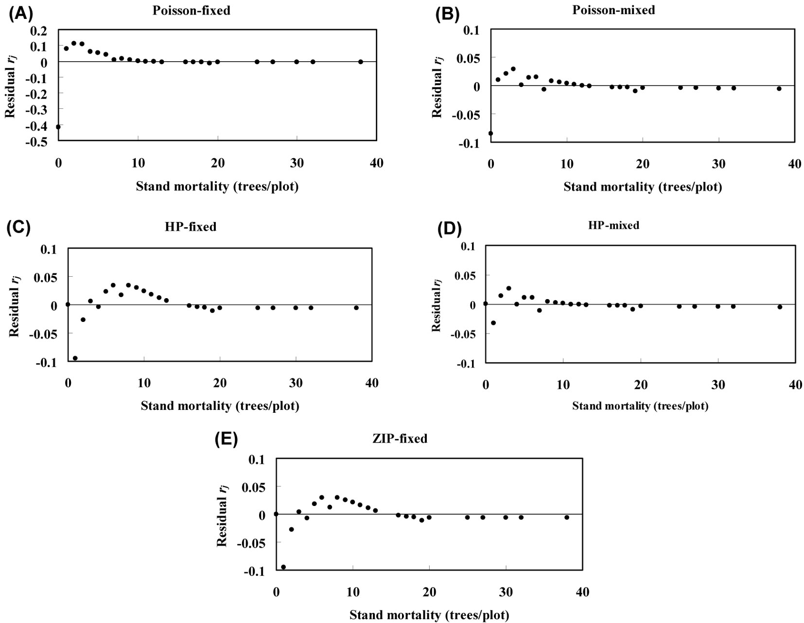
Additionally, the Vuong test-statistic V obtained from the comparison between the Poisson mixed-effects model and the Poisson fixed-effects model was 4.5, while a value V = 4.8 was estimated by comparing the HP mixed-effects model with the HP fixed-effects model. This means that models with random effects had better performances than fixed-effects models. We also compared the HP fixed-effects model with the ZIP fixed-effects model, remarking that the former model outperformed the latter (V = 5.0).
Overall, the best fit was detected for the HP fixed-effects and the HP mixed-effects model, therefore only these models were used in further analysis. Some variables with p>0.05 after the t-test were removed from the models (Tab. 3). In the positive count component of the models, all variables were significant at the 0.05 level (Tab. 3). Such variables have a meaningful biological interpretations in terms of tree mortality. Relative spacing is an indirect measure of the competition within the stand, being related to tree density (number of trees per hectare) and stand dominant height. According to previous studies ([7]), stand mortality decreases when the relative spacing is larger. Similarly, the effect of stand arithmetic mean diameter (size index) was negative (i.e., the greater Dm, the smaller stand mortality), indicating that stand mortality is more likely in forests with many small trees compared to forests with larger trees ([14]). Due to the random effects on plots, altitude was not significant in the mixed models (Poisson mixed-effects model, HP mixed-effects model). This may be because the random parameter explained the effects of altitude. In the zero component of the models, all the parameters listed in Tab. 3 were also significant at the 0.05 level. In this study, site quality (as reflected by the dominant height) was positively related with the probability of mortality. Accordingly, several studies reported a higher mortality in sites showing higher productivity ([33], [7]). On the other hand, Woollons ([31]) found that a higher mortality was related to lower site productivity. Therefore, site quality effects should be considered with caution before their inclusion in mortality models.
Tab. 3 - Estimations of parameters of the two model components in the HP fixed-effects and the HP mixed-effects models. (SE): standard error.
| Model Component |
Parameter | HP-fixed | HP-mixed | ||||
|---|---|---|---|---|---|---|---|
| Estimate | SE | p-value | Estimate | SE | p-value | ||
| Positive count component | Intercept | 4.0177 | 0.3249 | <0.001 | 6.2386 | 1.0851 | <0.001 |
| Rs | -1.5462 | 0.3091 | <0.001 | -3.3797 | 1.1974 | <0.01 | |
| Dm | -0.1187 | 0.0244 | <0.001 | -0.3171 | 0.0701 | <0.001 | |
| v | - | - | - | 1.764 | 0.5998 | <0.01 | |
| Zero component |
Intercept | -3.321 | 1.1945 | <0.01 | -3.321 | 1.1945 | <0.01 |
| H | 0.1846 | 0.0903 | <0.05 | 0.1846 | 0.0903 | <0.05 | |
| Rs | 4.7581 | 1.222 | <0.001 | 4.758 | 1.222 | <0.001 | |
In a tree mortality context, the use of HP models seems to be the most appropriate when applied to cases with no mortality, as it occurs in a stand before the competition among trees takes place. Once competitive pressures within the stand exceeds a certain threshold, positive mortality occurs consistently and in accordance with a ZIP probability mass function ([1]).
In our study, the application of both the above models led to the same qualitative results and gave very similar model fitting performances (Tab. 2, Fig. 3). These models have three main advantages. Firstly, by allowing distinct functions for the two components, the predicted stand mortality may be compared with that obtained assuming a Poisson-shaped data distribution. Secondly, the zero component and the positive count component of the two models may be directly interpreted in terms of the empirical features of the data. Thirdly, they perform better in modeling the data variability observed, therefore ensuring an appropriate use of the information collected ([3], [35]).
In this study, we used Poisson mixture model with mixed-effects to analyze stand mortality. Random-effects of both the Poisson model and HP model were significant at the 0.05 level. However, the ZIP model was not convergent after the random-effects were incorporated in the intercept of positive count component. Min & Agresti ([22]) found that fitting a ZIP random effect model was more complex than fitting a HP random effect model. Li et al. ([19]) incorporated the random effects in the count data models for analyzing tree in-growth, finding an improved model performance. Overall, both the Poisson and the HP model were largely improved by the inclusion of random effects, accounting for most of the variation among plots and data sources.
Acknowledgments
This work was carried out within the frame of the following projects: the Chinese State “TWELVE FIVE” Science and Technology Project (No. 2012BAD22B0201), and the “863” program from the Ministry of Science and Technology of China (No. 2012AA12 A306). The authors are grateful to two anonymous reviewers for their valuable suggestions and comments on an earlier version of the manuscript.
References
Gscholar
Gscholar
Gscholar
Authors’ Info
Authors’ Affiliation
Key Laboratory of Tree Breeding and Cultivation, State Forestry Administration, Research Institute of Forestry, Chinese Academy of Forestry, Beijing 100091 (China)
Xian-zhao Liu
Research Institute of Forest Resource Information Techniques, Chinese Academy of Forestry, Beijing 100091 (China)
Corresponding author
Paper Info
Citation
Zhang X-, Lei Y-, Liu X- (2015). Modeling stand mortality using Poisson mixture models with mixed-effects. iForest 8: 333-338. - doi: 10.3832/ifor1022-008
Academic Editor
Renzo Motta
Paper history
Received: Apr 26, 2013
Accepted: Jul 13, 2014
First online: Sep 05, 2014
Publication Date: Jun 01, 2015
Publication Time: 1.80 months
Copyright Information
© SISEF - The Italian Society of Silviculture and Forest Ecology 2015
Open Access
This article is distributed under the terms of the Creative Commons Attribution-Non Commercial 4.0 International (https://creativecommons.org/licenses/by-nc/4.0/), which permits unrestricted use, distribution, and reproduction in any medium, provided you give appropriate credit to the original author(s) and the source, provide a link to the Creative Commons license, and indicate if changes were made.

Web Metrics
Breakdown by View Type
Article Usage
Total Article Views: 54973
(from publication date up to now)
Breakdown by View Type
HTML Page Views: 45211
Abstract Page Views: 3663
PDF Downloads: 4568
Citation/Reference Downloads: 22
XML Downloads: 1509
Web Metrics
Days since publication: 4271
Overall contacts: 54973
Avg. contacts per week: 90.10
Article Citations
Article citations are based on data periodically collected from the Clarivate Web of Science web site
(last update: Mar 2025)
Total number of cites (since 2015): 19
Average cites per year: 1.73
Publication Metrics
by Dimensions ©
Articles citing this article
List of the papers citing this article based on CrossRef Cited-by.
Related Contents
iForest Similar Articles
Research Articles
Developing a stand-based growth and yield model for Thuya (Tetraclinis articulata (Vahl) Mast) in Tunisia
vol. 9, pp. 79-88 (online: 23 June 2015)
Research Articles
Estimation of stand crown cover using a generalized crown diameter model: application for the analysis of Portuguese cork oak stands stocking evolution
vol. 9, pp. 437-444 (online: 02 December 2015)
Research Articles
A geographically weighted deep neural network model for research on the spatial distribution of the down dead wood volume in Liangshui National Nature Reserve (China)
vol. 14, pp. 353-361 (online: 27 July 2021)
Research Articles
Developing stand transpiration model relating canopy conductance to stand sapwood area in a Korean pine plantation
vol. 14, pp. 186-194 (online: 14 April 2021)
Research Articles
Nonlinear mixed model approaches to estimating merchantable bole volume for Pinus occidentalis
vol. 5, pp. 247-254 (online: 24 October 2012)
Research Articles
Deriving tree growth models from stand models based on the self-thinning rule of Chinese fir plantations
vol. 15, pp. 1-7 (online: 13 January 2022)
Research Articles
Height-diameter models for maritime pine in Portugal: a comparison of basic, generalized and mixed-effects models
vol. 9, pp. 72-78 (online: 11 June 2015)
Research Articles
Spatio-temporal modelling of forest monitoring data: modelling German tree defoliation data collected between 1989 and 2015 for trend estimation and survey grid examination using GAMMs
vol. 12, pp. 338-348 (online: 05 July 2019)
Research Articles
Predictive capacity of nine algorithms and an ensemble model to determine the geographic distribution of tree species
vol. 15, pp. 363-371 (online: 20 September 2022)
Research Articles
Modelling the carbon budget of intensive forest monitoring sites in Germany using the simulation model BIOME-BGC
vol. 2, pp. 7-10 (online: 21 January 2009)
iForest Database Search
Search By Author
Search By Keyword
Google Scholar Search
Citing Articles
Search By Author
Search By Keywords
PubMed Search
Search By Author
Search By Keyword


