Assessing most relevant factors to simulate current annual increments of beech forests in Italy
iForest - Biogeosciences and Forestry, Volume 7, Issue 2, Pages 115-122 (2014)
doi: https://doi.org/10.3832/ifor0943-007
Published: Dec 31, 2013 - Copyright © 2014 SISEF
Research Articles
Abstract
Recent work of our research group demonstrated the applicability of a calibrated bio-geochemical model, BIOME-BGC, for estimating current annual increments (CAIs) of Mediterranean forests. In the current case, the model is applied to assess the gross primary production (GPP) of nine beech forest sites in Italy using a previously produced data set of meteorological data descriptive of a ten-year period (1999-2008). The obtained GPP estimates are integrated with relevant autotrophic respirations and allocations to derive forest net primary production (NPP) averages for the same forests. The simulations are performed assuming different levels of ecosystem disequilibrium, i.e. progressively taking into account the effects of specific site history in terms of woody biomass removal and stand aging.The NPP estimates, converted into CAIs by means of specific coefficients, are validated through comparison with data derived from tree growth measurements. Results indicate that the modelling of quasi-equilibrium conditions tends to produce overestimated CAI values, particularly for not fully stocked, old stands. The inclusion of information on existing biomass introduces a partial improvement, while optimal results are obtained when information on ecosystem development phase is considered. The implications of using different NPP estimation methods are finally discussed in the perspective of assessing the forest carbon budget on a national basis.
Keywords
CAI, NPP, Dendrochronological Data, Volume, Stand Age, BIOME-BGC
Introduction
Forests cover about one third of water-free land areas ([12]) and are important for timber production, recreational purposes, biodiversity conservation and erosion prevention. In addition, forests can act as carbon sink mitigating the consequences of climate changes ([10]). Given the increased importance of the above forest functions, the need for monitoring forest stocks not only on a local scale, as commonly done for commercial purposes, but also on a regional/global scale is currently felt by ecologists (e.g., [33]). More specifically, the spatio-temporal variations of forest carbon stocks and fluxes must be known in order to properly assess the land carbon balance on different spatial and temporal scales ([1], [28]). Efficient monitoring and reporting systems capable of quantifying variation of forest yields are therefore needed ([11]). Traditionally this objective has been fulfilled by the application of forest inventories, so as to obtain both basic forest attributes (e.g., basal area, stem volume, etc.) and current annual increment (CAI), defined as the mean woody biomass accumulated annually over a certain number of years (usually from five to ten). Forest inventories, however, require very expensive and time-consuming field surveys and cannot be carried out frequently ([33]).
An interesting alternative is the application of advanced methodologies quantifying forest production variations based on the combined use of remotely sensed data and bio-geochemical models. Maselli et al. ([20]) proposed an approach based on the biogeochemical model BIOME-BGC to simulate the CAI of forests in quasi-equilibrium with the climatic and edaphic conditions of each site. More specifically, calibrated versions of BIOME-BGC were applied to simulate photosynthesis, respiration and allocation processes for each forest type. In this way, most factors determining the spatio-temporal variation of CAI can be taken into account. Among these factors, the first to be considered is the composition in species, whose genetic and physiological characteristics strongly affect CAI variability ([2]). Moreover, knowledge of site conditions (i.e., the site index) is required, in that potential growth in each site and maximum tree development stems from the interaction between climate and soil. Other important factors are those related to biomass removal in each site, including the management practices applied (thinning and cutting operations), forest fires, diseases occurred, etc. Finally, the stand development stage must be taken into consideration, since forest production is strictly dependent on tree age (e.g., [16], [30], [36]). In fact, it is well known that old forests reduce their growth rate because of varying allocation properties (e.g., constant gross primary production - GPP - coupled with increasing respiration due to higher biomass), nutrient limitations, changes in hydraulic architecture, and decreased stand leaf area ([30]). The inclusion of all the mentioned factors within the proposed CAI modeling strategy can be carried out at different levels of complexity, depending on available input data and spatial and temporal scales of model application. This is expected to impact the accuracy of the model output in a way that has not yet been fully assessed.
The current paper aims at investigating the applicability of the model BIOME-BGC to assess current annual increments (CAIs) of nine beech forest sites spread over the Italian peninsula. Conventional forest measurements and tree growth data were fully available for all the sites considered. Moreover, various types of ancillary and remote sensing data were considered in the analysis. Data modeling was applied to obtain CAI estimates using progressively increasing information on each forest ecosystem (i.e., site condition, existing biomass and forest development phase). Finally, the accuracy of the CAI predictions obtained was tested by comparison to CAI measurements from tree growth data.
The paper is organized as follows. The main features of the selected forests are first described along with the ground and remote sensing data applied in the study. The modeling approach is then introduced, together with the steps used for its application and validation against available increment data. Next, the results are described and commented, with particular reference to examining the main sources of uncertainty in the evaluation of CAI. The paper is concluded by a section which highlights the potential contribution of the approach for the assessment of forest carbon budget on a national scale.
Study areas and data
Study areas
Beech (Fagus sylvatica L.) is a deciduous species widely distributed within European temperate forests, growing in environments relatively little affected by wildfires and characterized by a wide range of soil types. In Italy, it generally grows both on the Alps (generally at elevation > 500 m a.s.l.) and on the Apennines (elevation > 900 m a.s.l.).
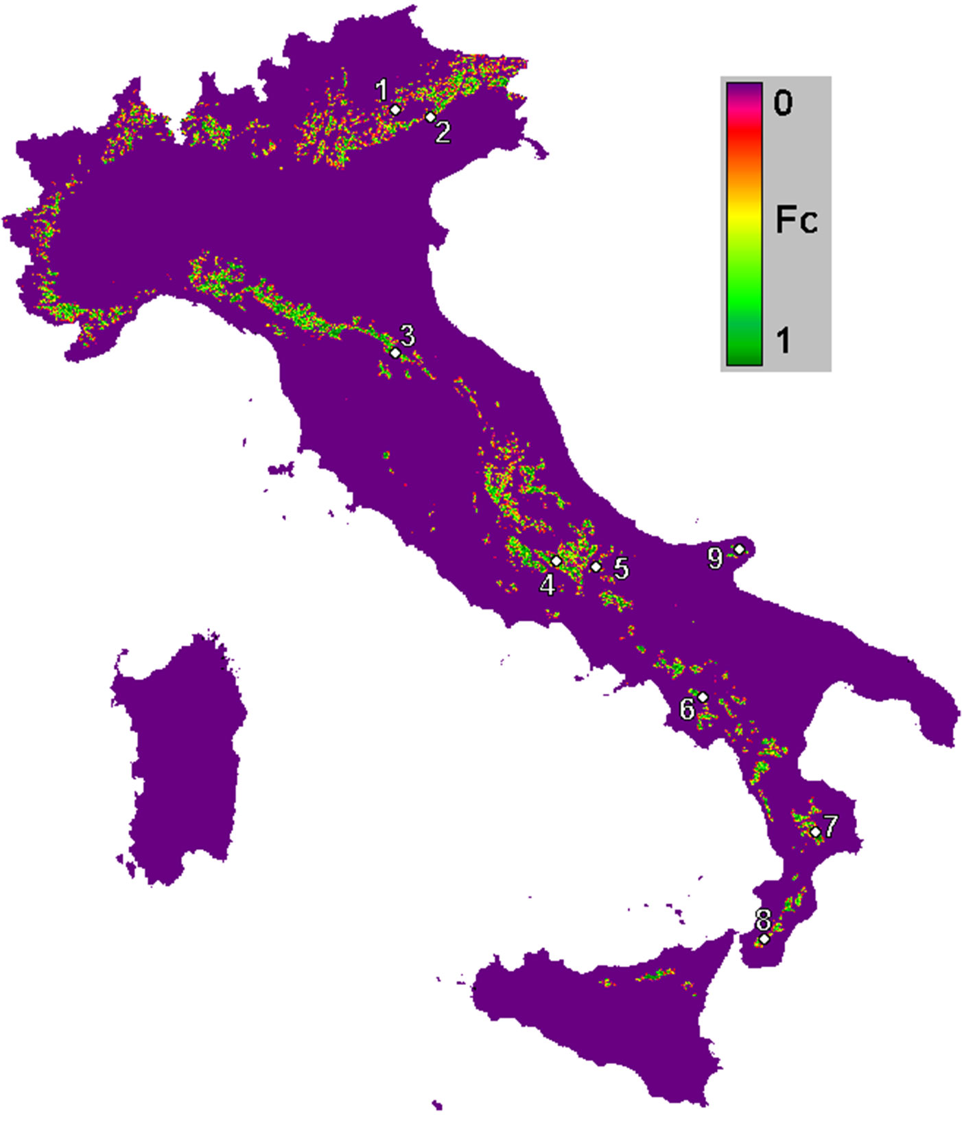
Nine beech forests were selected all over Italy (Fig. 1). Climate characteristics at the chosen locations vary from Mediterranean (south) up to temperate (north). The average annual temperature ranges from 7.5 °C in the north to 14.2 °C in the south; a trend of decreasing annual rainfall is observed moving from north to south, and from the highest to the lowest altitude of the sites (Tab. 1).
Fig. 1 - Fractional cover (Fc) of beech forests in Italy derived from the CORINE Land Cover 2006 (5°-20° Long. E, 36-48° Lat. N). White circles indicate the location of the nine beech forest sites considered in this study (the IDs refer to the site names reported in Tab. 1).
Tab. 1 - Main environmental characteristics of the beech forest sites studied. Meteorological data were derived from the downscaled E-OBS dataset (see text for more details).
| Study site | ID point | Geo-location (Long. E, Lat. N) |
Altitude (m a.s.l.) |
Average annual temp. (°C) |
Average annual rainfall (mm/y) |
|---|---|---|---|---|---|
| Dolomiti Bellunesi | 1 | 11.91, 46.12 | 1100 | 8.75 | 768.6 |
| Pian del Cansiglio | 2 | 12.38, 46.04 | 1300 | 7.5 | 974.47 |
| Sasso Fratino | 3 | 11.79, 43.84 | 1550 | 9.61 | 1708.97 |
| Val Cervara | 4 | 13.73, 41.83 | 1780 | 7.97 | 694.03 |
| Monte di Mezzo | 5 | 14.21, 41.75 | 1100 | 11.19 | 613.48 |
| Corleto | 6 | 15.42, 40.47 | 1130 | 11.67 | 655.73 |
| Sila | 7 | 16.65, 39.13 | 1680 | 9.89 | 806.26 |
| Aspromonte | 8 | 15.94, 38.17 | 1560 | 12.29 | 660.63 |
| Gargano | 9 | 16.01, 41.82 | 775 | 14.2 | 509.03 |
Meteorological and ancillary data
Meteorological information (i.e., daily minimum and maximum temperature and precipitation) for each site and for the period considered (1999-2008) was derived from the E-OBS dataset ([17]). Data are freely provided at the original spatial resolution of 0.25° and were then downscaled at 1-km spatial resolution by applying locally calibrated regressions after Maselli et al. ([23]).
A field survey was carried out at each site to determine the actual standing volume by directly measuring diameter at breast height (DBH) and height of trees standing within circular plots of varying radius (Tab. 2).
Tab. 2 - Characteristics of the dendrochronological measurements.
| Study site | Length of the data series |
Average tree ring width (mm/y) |
Volume (m3/ha) |
CAI (m3/ha) |
|---|---|---|---|---|
| Dolomiti Bellunesi | 1915-2006 | 2.24 | 380 | 5.26 |
| Pian del Cansiglio | 1814-2008 | 2.18 | 791 | 8.22 |
| Sasso Fratino | 1827-2008 | 2.1 | 985 | 8.94 |
| Val Cervara | 1715-2008 | 0.92 | 364 | 1.48 |
| Monte di Mezzo | 1844-2004 | 2.62 | 703 | 7.8 |
| Corleto | 1821-2006 | 1.98 | 832 | 12.68 |
| Sila | 1854-2008 | 2.14 | 775 | 10.81 |
| Aspromonte | 1824-2008 | 1.87 | 687 | 2.07 |
| Gargano | 1827-2008 | 1.82 | 632 | 6.23 |
Tree growth data
For each site, tree growth measurements were collected and elaborated as dendrochronological series in order to retrieve reference CAI values (see Tab. 2). At each site, an area of approximately 2 ha was chosen and 15-16 living dominant and co-dominant trees were selected, with DBH ranging from 60 to 100 cm and height about 26 m. Care was taken to select trees with canopies well separated from each other, in order to reduce the effect of competition on tree growth. Two cores were taken by an increment borer 0.5 cm in diameter from each tree, uphill at height of 1.3 m at an angle of 120° to each other. Cores were mounted on channeled wood, seasoned in a fresh-air dry store and sanded a few months later. Tree rings were dated by counting them from bark to pith. Ring widths were measured to the nearest 0.01 mm using the LINTAB-measurement equipment, coupled to a stereomicroscope (60x magnification - Leica, Germany). The Time Series Analysis Programme (TSAP) software package (Frank Rinn, Heidelberg, Germany) was used for statistical analysis. Raw ring widths of the single series of each dated tree were cross-dated statistically by the percent agreement in the signs of the first-differences of the two time series (the Gleichlaufigkeit, GLK - [18]). The GLK is a measure of the year-to-year agreement between the interval trends of two chronologies based upon the sign of agreement, or the sum of the equal slope intervals in per cent. With an overlap of 50 years (commonly used in tree-ring studies), GLK becomes significant (p < 0.05) at 62% and highly significant (p < 0.01) at 67%. With an overlap of 10 years, GLK becomes significant (p < 0.05) at 76% and highly significant (p < 0.01) at 87% ([18]). In this study, most time series analyzed were longer than 50 years and cross dating was considered successful if GLK was higher than 60%.
The statistical significance of the GLK (GSL) was also computed. The TVBP, a Student’s t-value modified by Baillie & Pilcher ([3]) was used for investigating the significance of the best match identified. The TVBP is commonly used as a statistical tool for comparing and cross-dating ring widths series. It determines the degree of correlation between curves and eliminates low-frequency variations in the time series, as each value is divided by the corresponding 5-year moving average.
Locally missing or discontinuous rings were identified by cross-dating the two tree-ring cores obtained from the same tree. Standard methods ([14]) were used to build a tree averaged series and the mean chronologies of the investigated sites, using ring-width series obtained from all living trees growing at each study site.
Modeling approach
The methodology developed by our research group allows the calibration of the BIOME-BGC model for each main forest type ([5]). This is obtained by iteratively adapting the GPP estimates of the model to those of a Monteith’s type, NDVI-driven parametric model, Modified C-Fix, whose accuracy has been widely tested against eddy covariance flux tower measurements ([21], [6]). Next, BIOME-BGC is applied for each forest site to simulate all main forest processes ([20]). In the current paper only the main steps of the methodology are summarized. Theoretical and operational details can be found in the references mentioned below.
BIOME-BGC, after a proper calibration for beech (see [7]), is capable of estimating respiration and allocation processes of ecosystems close to equilibrium condition ([9], [37]). For each study site the model can perform a self-initialization through the so-called spin-up phase, which identifies the initial state variables. In this way, the model can predict the net forest carbon fluxes depicting a quasi-equilibrium situation. More specifically, net primary production (NPP) is obtained as follows (eqn. 1):
where GPP, Rg and Rm correspond to the annual gross primary production, growth and maintenance respiration simulated by BIOME-BGC (g C m-2 year-1), respectively.
From NPP, CAI (m3 ha-1 year-1) can be predicted through the general formula (eqn. 2):
where SCA corresponds to the stem carbon allocation, BEF is the biomass expansion factor and BWD is the basic woody density. The SCA for beech is derived from the BIOME-BGC settings ([38], [7]), while BEF and BWD are 1.36 and 0.61, respectively ([13]). The two scalars 2 and 100 are applied to convert CAI from carbon to dry matter and from g m-2 to Mg ha-1, respectively.
The effects of forest disturbances on NPP can be taken into account by applying the methodology proposed by Maselli et al. ([20]): the ratio between actual and potential tree volume is considered as an indicator of ecosystem proximity to potential biomass density, which can be used to correct the GPP and respiration estimates obtained by the previous model simulations. According to this formulation, actual forest NPP (NPPA, g C m-2 year-1) can be approximated as follows (eqn. 3):
where the two dimensionless terms FCA (actual forest cover) and NVA (actual normalized standing volume) are derived from the ratio between actual and potential tree volume ([20]).
The above modification works as depicted in Fig. 2a. Simulated CAI starts from 0 (no woody biomass) and increases as function of the stand volume up to a maximum value, which is slightly higher than BIOME-BGC (equilibrium) CAI due to the reduced influence of autotrophic respiration. Next, when actual biomass approaches potential biomass, respiration increases and simulated CAI tends to reach the CAI simulated by BIOME-BGC.
Fig. 2 - Effects of biomass (a) and age (b) variations on simulated CAIs. Both curves are relative to BIOME-BGC CAI modeling at equilibrium conditions and are derived from Maselli et al. ([20]) and Chiesi et al. ([8]), respectively; in the latter case a stem volume lower than the potential maximum is considered (see text for details).
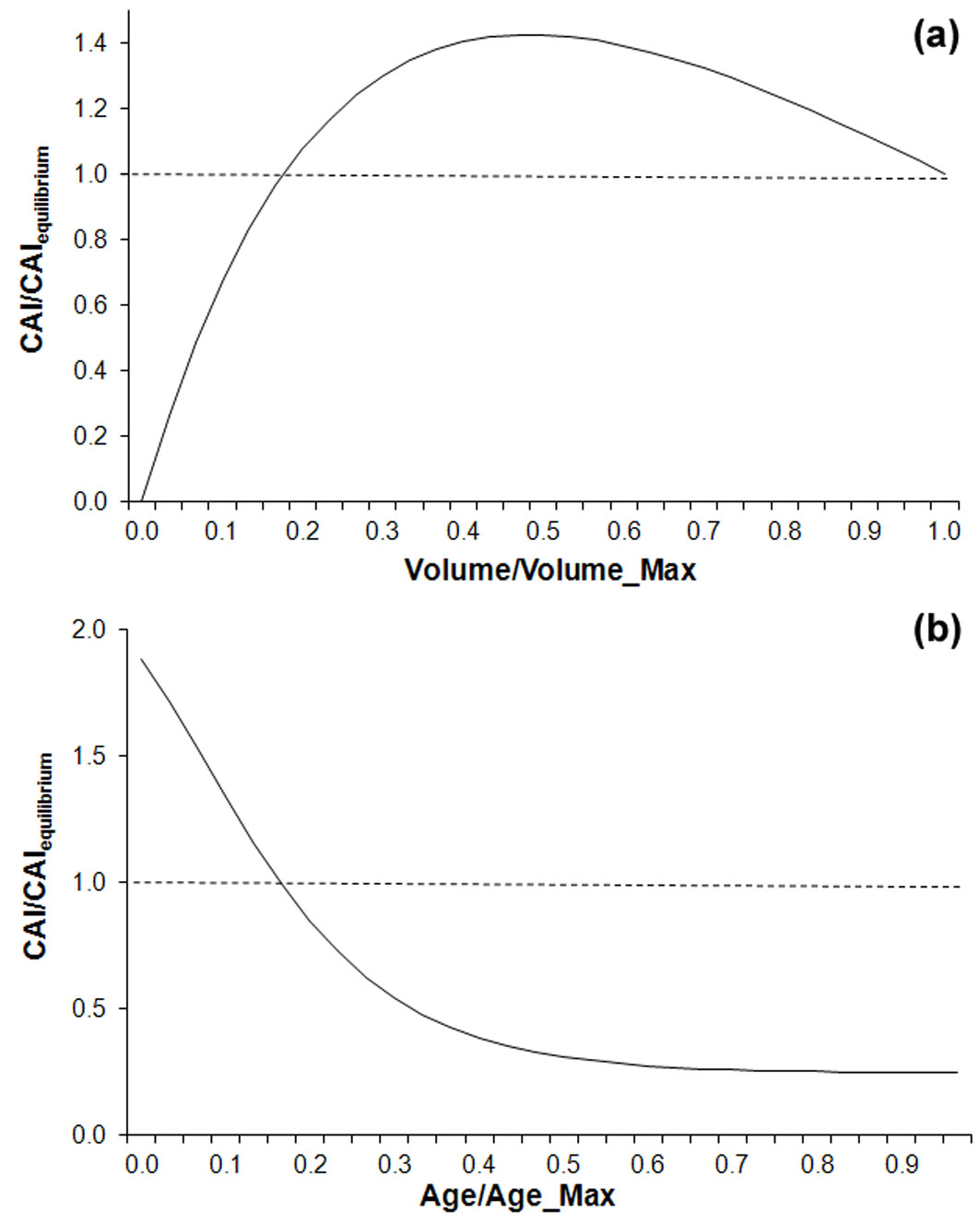
The strategy has been further refined to take into consideration the age-related growth decline typical of even-aged stands ([8]). This is obtained using an age-dependent relationship between stem carbon and leaf carbon, which must be calibrated for each study site and transforms FCA into FCEA (even-aged actual forest cover). Accordingly, even-aged NPP (NPPEA) is obtained as follows (eqn. 4):
As fully explained by Chiesi et al. ([8]), applying the above equation leads to modify the relationship between photosynthesis and autotrophic respiration in an age-dependent way. Consequently, for a certain woody biomass, tree aging has an inhibiting effect on the predicted CAI. This is schematized in Fig. 2b, where the ratio between aging CAI and BIOME-BGC (equilibrium) CAI is much higher than 1 for young stands and tends to decrease and level off for older stands.
Data processing
Elaboration of dendrochronological data series
Dendrochronological measurements (i.e., annual tree ring widths) collected in each forest site were elaborated to retrieve forest volume variations during the stand development since the planting date. To this aim, the DBH was first reconstructed by summing up the tree ring widths. A cubic function was then applied to retrieve the stem volume corresponding to each diameter measurement ([31]). This volume was then normalized against the actual forest volume measured in the field (see Tab. 1). The annual CAIs were finally calculated as the difference between the stem volumes of two successive years. To validate the simulation methods, reference CAI values were obtained for each of the nine sites considered by averaging the annual CAI over the last five years available.
Simulation of forest CAIs
First, the input layers required to apply the BIOME-BGC model were prepared. The 1-km spatial resolution minimum and maximum temperature and precipitation data for the years 1999-2008 (see above) were further elaborated to obtain solar radiation by using the MT-CLIM algorithm ([32]).
The modeling strategy was first applied to simulate ecosystems in equilibrium conditions. In particular, BIOME-BGC was applied using the ecophysiological parameters reported by Chiesi et al. ([7]), and NPP and CAI were predicted using eqn. 1 and eqn. 2.
Next, the effects of biomass removal were obtained by applying eqn. 3. In particular, both NVA and FCA were calculated using the measured stem volume for each stand (see Tab. 2). NVA was the ratio between actual and potential stem volume, while FCA was computed using the maximum stand LAI (see [20] for more details).
Finally, the effects of stand aging were simulated using both a unique modeling of the leaf carbon/stem carbon temporal variability and site specific modeling of the same variability using eqn. 4 (see [8] for details). In the first case, a general growth curve was calibrated by statistically reproducing the average of all available reference CAIs derived from dendrochronological measurements with the exclusion of the last 5 years; this allowed an approximate independence of the calibration and validation phases. As for the second case, the same calibration process was repeated by fitting a specific growth curve for each study site.
In all cases, the obtained CAI estimates were averaged over the 5 study years and compared to the reference CAI measurements using the correlation coefficient (r), the root mean square error (RMSE) and the mean bias error (MBE) as accuracy statistics.
Results
The study sites are located in mountain areas at elevations ranging between 775 and 1780 m a.s.l. As a consequence of different latitudes and elevations, the annual average air temperature and the total annual precipitation derived from the downscaled E-OBS dataset are highly variable: air temperature ranges between 7.5 °C and 14.2 °C, while precipitation ranges between 510 mm y-1 and 1710 mm y-1 - Tab. 1).
The beech forests analyzed show different structural characteristics, which are related to the different age of trees. Tab. 2 reports the average tree ring widths, which vary between 0.92 and 2.62 mm y-1, where the oldest stand shows the lowest tree ring width (Val Cervara). The same general trend is observed for CAI measurements, which range between 1.5 and 12.7 m3 ha-1, depending on different environmental conditions, structures and development phases of the nine study sites considered.
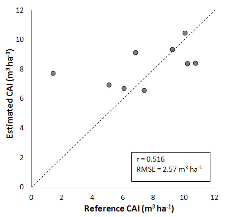
Results shown in Fig. 3 are obtained using the BIOME-BGC GPP, respirations and allocations for forests in quasi-equilibrium with site-specific climatic and soil conditions. The correlation between measured and predicted CAIs is moderate (r = 0.516), and the range of variation was strongly underestimated. CAI is particularly overestimated for Val Cervara (7.79 vs. 1.41 m3 ha-1), which is the less dense and oldest stand (see Tab. 2). This leads to a relatively high overall RMSE (2.57 m3 ha-1), indicating that the exclusion of actual forest conditions (in terms of existing biomass and development phase) implies a flawed simulation of CAI variations.
Fig. 3 - Comparison between CAI measured and estimated using BIOME-BGC simulation of equilibrium (quasi-climax) forest conditions (see text for details).
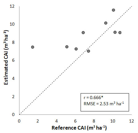
A slight improvement is obtained including the information on the existing stem volume into the model. The comparison between measured and estimated CAI is shown in Fig. 4. CAI overestimation for Val Cervara reported in Fig. 3 is marginally reduced, and the global estimation accuracy is slightly increased (r = 0.666, RMSE = 2.53 m3 ha-1).
Fig. 4 - Comparison between CAI measured and estimated by including volume information about each site (see text for details). (*): significant correlation, P < 0.05.
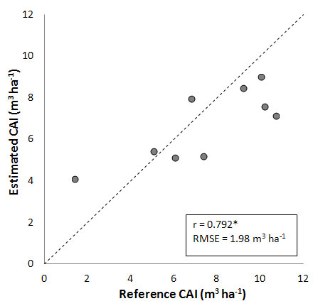
Further improvements in predictions are obtained when the stand development stage is included in the model, based on the available dendrochronological measurements and the method reported by Chiesi et al. ([8]). More specifically, the use of a generic growth curve for all beech forests yields the results shown in Fig. 5. The correlation coefficient is notably increased (r = 0.792), and the error markedly reduced (RMSE = 1.98 m3 ha-1). Indeed, the inclusion of generic information on beech stand development reduces the former overestimation for Val Cervara, though a slight underestimation at high CAI values is observed.
Fig. 5 - Comparison between CAI measured and estimated by applying a generic age-dependent growth curve (see text for details). (*): significant correlation, P < 0.05.
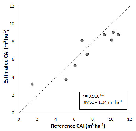
An additional improvement in simulations is obtained when locally derived growth curves are calibrated to better characterize the specific stand development phase of each site (Fig. 6). In this case, reference CAIs are fairly well simulated for all study sites considered, with a high correlation coefficient (r = 0.916), and a RMSE strongly reduced (1.34 m3 ha-1).
Fig. 6 - Comparison between CAI measured and estimated by applying an age-dependent growth curve calibrated for each single stand (see text for details). (**): highly significant correlation, P < 0.01.
Discussion and conclusions
Several recent papers have demonstrated that a modeling strategy based on the use of a calibrated bio-geochemical model is capable of predicting gross and net forest carbon fluxes within Mediterranean forests (e.g., [26], [34], [20], [22], [6], [8]). Modeling can be applied at different levels of complexity, depending on the existing knowledge of the forest ecosystems considered. This is expected to affect the accuracy of the proposed strategy in a way that is important to be assessed in sight of operational monitoring applications.
The current study investigates on this issue using ground and remote sensing information collected over nine beech sites in Italy. The availability of dendrochronological sequences of tree ring-widths has allowed a thorough characterization of the past and present growth status of the considered forest stands, providing essential information for both calibrating and validating the modeling simulations.
In general, the accuracy of the modeling strategy is affected by the uncertainty of the input data used. While a full assessment of this topic has been performed in previous papers (e.g., [6], [23]), the critical nature of the extended meteorological model drivers must be highlighted. This is particularly the case for the daily rainfall estimates, whose accuracy is relatively low due to a number of problems ([23]).
The proposed use of BIOME-BGC allows to reproduce the carbon accumulated by forests which are in quasi-equilibrium with local climatic and soil conditions. This means that the annual net fluxes are close to zero because of the nearly equivalence of forest production and respiration; additionally, such models simulate forests composed by trees in different growing phases ([29], [20]). The model can be applied in a relatively simple way, requiring only information on forest types and eco-climatic conditions, which is now available for the European continent from several sources (e.g., [27], [17]). On the other hand, the exclusion of biomass removal and stand aging from the model usually leads to underestimate the range of CAI variations ([20], [8]). As reported in Fig. 2, the two factors above can increase or decrease the simulated CAI depending on the ecosystem closeness to potential, quasi-equilibrium condition.
The additional inclusion of a proxy of the ecosystem distance from equilibrium (i.e., the stand volume information) accounts for the effect of biomass removal and generally improves the simulation results ([20]). However, the forests examined in this study are nearly fully stocked and old growth, which reduces the effect of biomass removal and enhances that of age-related decline in forest production ([16], [8]). The latter factor is not accounted for by this modeling step, which therefore improves the predictions only marginally. A different situation would occur in uneven-aged stands having biomass much lower than potential; in such a case, the inclusion of biomass removal into the model would be decisive for CAI simulation ([22]). From an operational point of view, including the information on the existing biomass makes the application of the simulation method more complex, since spatially distributed estimates of stem volume are usually difficult to retrieve. Efforts in this direction, however, have been recently performed. For example, Gallaun et al. ([15]) produced and disseminated a 1-km stem volume map covering all European forest areas. Maselli et al. ([25]) performed a similar effort for the Italian territory by combining ground stem volume measurements with optical and LiDAR satellite data.
According to the previous considerations, an additional methodological improvement is provided by modeling the effects of stand aging. In fact, tree aging leads to decreased accumulation rates due to the well-known phenomenon of age-related decline in forest production (e.g., [16], [4]). The causes of this phenomenon are numerous and mainly related to environmental and external factors (e.g., silvicultural practices, forest fires, etc. - [39]). The availability of dendrochronological measurements enables to characterize the whole stand development of the beech forests and to reconstruct the temporal variations of CAI with stand age. This was obtained by defining an age-dependent relationship between leaf carbon and stem carbon accounting for the temporally varying ratios between forest production and respiration related to changes in canopy density, tree competition and allocation patterns.
In the current study this operation has been carried out in two steps: first, applying a general relationship between leaf carbon and stem carbon; and, second, using a site-specific relationship. This has improved the accuracy of the estimates especially in the latter case (r = 0.916 - see Fig. 6). In addition to a few dendrochronological tree ring-width sequences, the application of the first methodological step would require spatially distributed estimates of stand age. Efforts in this direction have been recently performed: Vilén et al. ([35]), for example, produced and disseminated a 1-km map of forest age covering all Europe.
For relatively small areas an alternative could be provided by tree height estimates obtained from LiDAR data, which can be used as a proxy of tree age ([24]), though old small individuals and, vice-versa, trees with huge biomass accumulated in few decades, can be found in forest ecosystems ([19]). Finally, as regards the last step, its application on regional to national scales is virtually unfeasible, since the dendrochronological measurements needed to characterize specific site history can be obtained only for small areas.
In summary, the current study has shown that the inclusion of progressively increasing information levels on forest conditions within the model allows to obtain reliable predictions of stand CAI over large areas. However, the complete simulation of the effects of human induced factors requires a full characterization of specific site history, which is practically unfeasible over large areas. Consequently, a certain approximation must be accepted for operational applications, depending on the spatio-temporal scales considered and on the nature and accuracy of the available datasets.
Acknowledgments
The Italian Ministry of Education, University and Research funded this study under the FIRB2008 program, project “Modelling the carbon sink in Italian forest ecosystems using ancillary data, remote sensing data and productivity models” C_FORSAT (code: RBFR08LM04, national coordinator: G. Chirici).
The authors acknowledge the E-OBS dataset from the EU-FP6 project ENSEMBLES (⇒ http://ensembles-eu.metoffice.com/) and the data providers in the ECA&D project (⇒ http://eca.knmi.nl/). The authors also wish to thank Dr. M. Pasqui for pre-processing the data from the E-OBS dataset, Dr. L. Fibbi, Dr. M. Moriondo and Prof. M. Bindi for assisting in the calibration and application of BIOME-BGC.
The authors wish to thank two anonymous reviewers for their precious comments on the first draft of the manuscript.
References
CrossRef | Gscholar
Gscholar
Gscholar
CrossRef | Gscholar
Gscholar
Gscholar
CrossRef | Gscholar
CrossRef | Gscholar
Gscholar
Gscholar
Gscholar
Authors’ Info
Authors’ Affiliation
Fabio Lombardi
Roberto Tognetti
Marco Marchetti
Dipartimento di Bioscienze e Territorio (DIBT), University of Molise, c.da Fonte Lappone, I-86090 Pesche (Italy)
Consiglio per la Ricerca e la Sperimentazione in Agricoltura, Forestry Research Centre (CRA-SEL), v.le Santa Margherita 70, I-01100 Arezzo (Italy)
The EFI Project Centre on Mountain Forests (MOUNTFOR), Fondazione Edmund Mach, v. Edmund Mach, I-38010 San Michele all’Adige (Italy)
Corresponding author
Paper Info
Citation
Chiesi M, Maselli F, Chirici G, Corona P, Lombardi F, Tognetti R, Marchetti M (2014). Assessing most relevant factors to simulate current annual increments of beech forests in Italy. iForest 7: 115-122. - doi: 10.3832/ifor0943-007
Academic Editor
Giorgio Matteucci
Paper history
Received: Jan 04, 2013
Accepted: Nov 22, 2013
First online: Dec 31, 2013
Publication Date: Apr 02, 2014
Publication Time: 1.30 months
Copyright Information
© SISEF - The Italian Society of Silviculture and Forest Ecology 2014
Open Access
This article is distributed under the terms of the Creative Commons Attribution-Non Commercial 4.0 International (https://creativecommons.org/licenses/by-nc/4.0/), which permits unrestricted use, distribution, and reproduction in any medium, provided you give appropriate credit to the original author(s) and the source, provide a link to the Creative Commons license, and indicate if changes were made.

Web Metrics
Breakdown by View Type
Article Usage
Total Article Views: 56294
(from publication date up to now)
Breakdown by View Type
HTML Page Views: 47048
Abstract Page Views: 2959
PDF Downloads: 4738
Citation/Reference Downloads: 70
XML Downloads: 1479
Web Metrics
Days since publication: 4517
Overall contacts: 56294
Avg. contacts per week: 87.24
Article Citations
Article citations are based on data periodically collected from the Clarivate Web of Science web site
(last update: Mar 2025)
Total number of cites (since 2014): 10
Average cites per year: 0.77
Publication Metrics
by Dimensions ©
Articles citing this article
List of the papers citing this article based on CrossRef Cited-by.
Related Contents
iForest Similar Articles
Review Papers
Remote sensing-supported vegetation parameters for regional climate models: a brief review
vol. 3, pp. 98-101 (online: 15 July 2010)
Review Papers
Accuracy of determining specific parameters of the urban forest using remote sensing
vol. 12, pp. 498-510 (online: 02 December 2019)
Review Papers
Remote sensing of selective logging in tropical forests: current state and future directions
vol. 13, pp. 286-300 (online: 10 July 2020)
Technical Reports
Detecting tree water deficit by very low altitude remote sensing
vol. 10, pp. 215-219 (online: 11 February 2017)
Research Articles
Assessing water quality by remote sensing in small lakes: the case study of Monticchio lakes in southern Italy
vol. 2, pp. 154-161 (online: 30 July 2009)
Research Articles
Use of BIOME-BGC to simulate water and carbon fluxes within Mediterranean macchia
vol. 5, pp. 38-43 (online: 02 April 2012)
Research Articles
Afforestation monitoring through automatic analysis of 36-years Landsat Best Available Composites
vol. 15, pp. 220-228 (online: 12 July 2022)
Review Papers
Remote sensing support for post fire forest management
vol. 1, pp. 6-12 (online: 28 February 2008)
Technical Reports
Remote sensing of american maple in alluvial forests: a case study in an island complex of the Loire valley (France)
vol. 13, pp. 409-416 (online: 16 September 2020)
Research Articles
Geostatistical techniques for estimating aboveground biomass in eastern Amazonia
vol. 19, pp. 85-93 (online: 13 March 2026)
iForest Database Search
Search By Author
Search By Keyword
Google Scholar Search
Citing Articles
Search By Author
Search By Keywords
PubMed Search
Search By Author
Search By Keyword


