Large scale semi-automatic detection of forest roads from low density LiDAR data on steep terrain in Northern Spain
iForest - Biogeosciences and Forestry, Volume 12, Issue 4, Pages 366-374 (2019)
doi: https://doi.org/10.3832/ifor2989-012
Published: Jul 05, 2019 - Copyright © 2019 SISEF
Research Articles
Abstract
While forest roads are important to forest managers in terms of facilitating the exploitation of wood and timber, their role is far more multifunctional. They permit access to emergency services in the case of forest fires as well as acting as fire breaks, enhance biodiversity, and provide access to the public to enjoy recreational activities. Detailed maps of forest roads are an essential tool for better and more timely forest management and automatic/semi-automatic tools allow not only the creation of forest road databases, but also enable these to be updated. In Spain, LiDAR data for the entire national territory is freely available, and the capture of higher density data is planned in the next few years. As such, the development of a forest road detection methodology based on LiDAR data would allow maps of all forest roads to be developed and regularly updated. The general objective of this work was to establish a low density LiDAR data-based methodology for the semi-automatic detection of the centerline of forest roads on steep terrain with various types of canopy cover. Intensity and slope images were generated using the currently available LiDAR data of the study area (0.5 points m-2). Two image classification approaches were evaluated: pixel-based and object-oriented classification (OBIA). The LiDAR-derived centerlines obtained with the two approaches were compared with the real centerlines which had previously been digitized in the field. The road width, type of surface and type of vegetation cover were also recorded. The effectiveness of the two approaches was evaluated through three quality indicators: correctness, completeness and quality. In addition, the accuracy of the LiDAR-derived centerlines was also evaluated by combining GIS analysis and statistical methods. The pixel-based approach obtained higher values than OBIA for two of the three quality measures (correctness: 93% compared to 90%; and quality: 60% compared to 56%) as well as in terms of positional accuracy (± 5.5 m vs. ± 6.8 for OBIA). The results obtained in this study demonstrate that producing road maps is among the most valuable and easily attainable products of LiDAR data analysis.
Keywords
GIS, Pixel-based Classification, OBIA, Quality Measures, Forest Roads Network, Accuracy Assessment
Introduction
The forest road network comprises roadways within the forest which are used for access or for timber extraction, an infrastructure which, among other things, is essential for carrying out the sustainable management of forests ([22]). Forest road networks provide connections between different forested areas as well as to the primary road network, thereby providing access to recreational and educational activities for the public, as well as playing an important role in fire-fighting support (both preventative in terms of forest roads acting as firebreaks and in terms of access to emergency services in the case of forest fires) and logging activities ([20]). Despite this, it must also be acknowledged that forest roads can also have negative impacts on the health of ecosystems, mainly in relation to hydrology and habitat disturbance ([35]).
From the point of view of forestry production, in order to carry out profitable and sustainable forest management it is crucial to create management tools that help to establish the availability of resources and the economic viability of their use, so that logging costs can be minimized. To efficiently calculate transport costs (including hauling and road transport phases), it is essential to have access to information on the extent and conditions of the current road forest network. The role of GIS (Geographical Information Systems) in this respect is increasingly important and such data can provide a solid framework for forestry companies seeking to improve their logistics, as it allows the optimization of transport planning according to various criteria ([2]). For all the reasons mentioned above, it is essential to develop automatic/semi-automatic tools to enable forest roads and timber extraction routes mapping as well as their periodic updating.
In general terms, the task of detecting and extracting the course of roads from digital information has been addressed in a number of ways over the years: photointerpretation and manual digitization, the integration of cartography from different sources, data capture in the field, and data capture from remote sensors ([27]). In the case of spatial data sources (aerial photographs or satellite images), the application of image classification methods for road extraction has been studied for more than twenty years ([21], [23], [11], [32], [27]). However, these methodologies all suffer similar problems with respect to field data collection in relation to forest roads: (i) the high cost of data acquisition in relation to the relatively small areas that can be mapped; (ii) interference of GPS signal; and (iii) occlusions due to the presence of trees ([1]). With the techniques of photointerpretation and remote sensing the main drawbacks are the resolution of the produced images, which in some cases is not sufficient for the detection of very narrow carriageways, and difficulty in obtaining information from below tree covered areas, which leads to discontinuities in the centerlines of the forest roads identified ([35]).
Within this unfavorable context for the application of remote sensing images in forest areas, LiDAR technology brought about a great advance in the automatic detection and updating of forest road networks, because it provides accurate measurements of ground elevation, which allows high resolution topographic mapping, even under dense canopy cover ([39]). As such, forest roads are easy to identify as they are on ground level, have a different topographic profile to other environments (planarity of the road surface) and present high spectral contrast with the otherwise undisturbed environment. These attributes can be exploited through the analysis of LiDAR point clouds and LiDAR intensity values ([5]). Various authors have already harnessed the great potential of LiDAR data for forest road detection and used airborne laser scanning devices in studies using a variety of approaches. In terms of how roads are represented in the final data collected, remote sensing methods can be grouped into those that produce two-dimensional elements (road segments) and those that produce one-dimensional lines (road centerline - [7]). Typically, research in the first group uses high resolution/density data and allows the detection of both the length and width of forest roads. Some examples are the method based on standard edge extraction algorithms from the slope map ([7]), the object-oriented classification developed by Sherba et al. ([35]) and the Support Vector Machine used by Azizi et al. ([3]). In contrast, studies in the second group use low resolution/density data which allows the detection of the road centerline, and include, for example, the dynamic programming method proposed by Saito et al. ([34]).
In general, while Saito et al. ([34]) achieved good results in terms of number of roads detected and the accuracy of their centerlines with high or medium density data, all methods encounter difficulties in areas of dense canopy covers, and where there is a high degree of slope and the density of ground points on roads obscured by dense vegetation will be much lower. Thus, methods that are based on the assumption that roads will have a higher density of ground points than forested areas, such as the one developed by Beck et al. ([4]), may fail in detecting roads lined by dense tree cover. On the other hand, on steep terrain, the filtering algorithms have problems distinguishing which elevation is actually the ground level. Since the methods of forest road extraction developed to date ([7], [3]) have used DTMs (Digital Terrain Models), which are based on ground point information, this entails a challenge for forest road detection using LiDAR data. In addition, the limited availability of LiDAR data hampers the development of comprehensive forest road network maps, since data acquisition is one of the most expensive steps in remote sensing studies ([18]).
In this respect, Spain is one of the few countries in the world to have a National Plan for Territory Observation (LiDAR-PNOA© National Geographic Institute of Spain) which ensures the capture of LiDAR data at various times across the whole of its territory. At the moment, data from only one flight (between 2008 and 2015, depending on the region) is available for civil use, but more flights to update the current data are expected to take place in the next couple of years. While this data has one main drawback - the low cloud point density used for the vast majority of the territory (only 0.5 points m-2) - this is counterbalanced by the fact that data is available for the whole national territory at no cost. In addition, the fact that the data is to be updated periodically with further flights means that there is an ongoing source of date to use to ensure that the mapping of the forest road network is regularly brought up to date.
Despite the easily accessible availability of LiDAR data and the great potential that this technology has shown in various studies, in Spain no great efforts have been made to build a public cartography of forest road networks. This fact is especially worrisome in the northern part of the country (specifically in Asturias) where according to the Spanish National Forest Inventory ([12]), 73% of the total surface is forested and the potential for wood production is extremely high. Within this area, however, environment conditions are difficult, i.e., very steep orography (47% of the land covered by trees has a slope between 30 and 60% while 5% has more than 60%) and densely planted forest stands.
In view of the above, this study aims to test the hypothesis that it possible to use low-density LiDAR data to semi-automatically detect and extract forest roads and that this is a more efficient alternative than manual digitization. The study aims to design a semi-automatic methodology to obtain the centerline of forest roads from low density LiDAR data in a steep forested environment. Two approaches have been evaluated: a pixel-based methodology and one which is object-oriented (OBIA). In addition, the influence of the characteristics of forest roads (width and type of road surface) and the surrounding vegetation (type of canopy cover bordering the road) on the results of these two types of semi-automated detection was also analyzed. Steep environments are acknowledged to be an extremely difficult context for forest management ([39]) and to obtain accurate information about forest road networks, thus a method of road detection that is effective and efficient in these conditions is likely to be easily applied in less challenging circumstances.
Material and methods
Study area
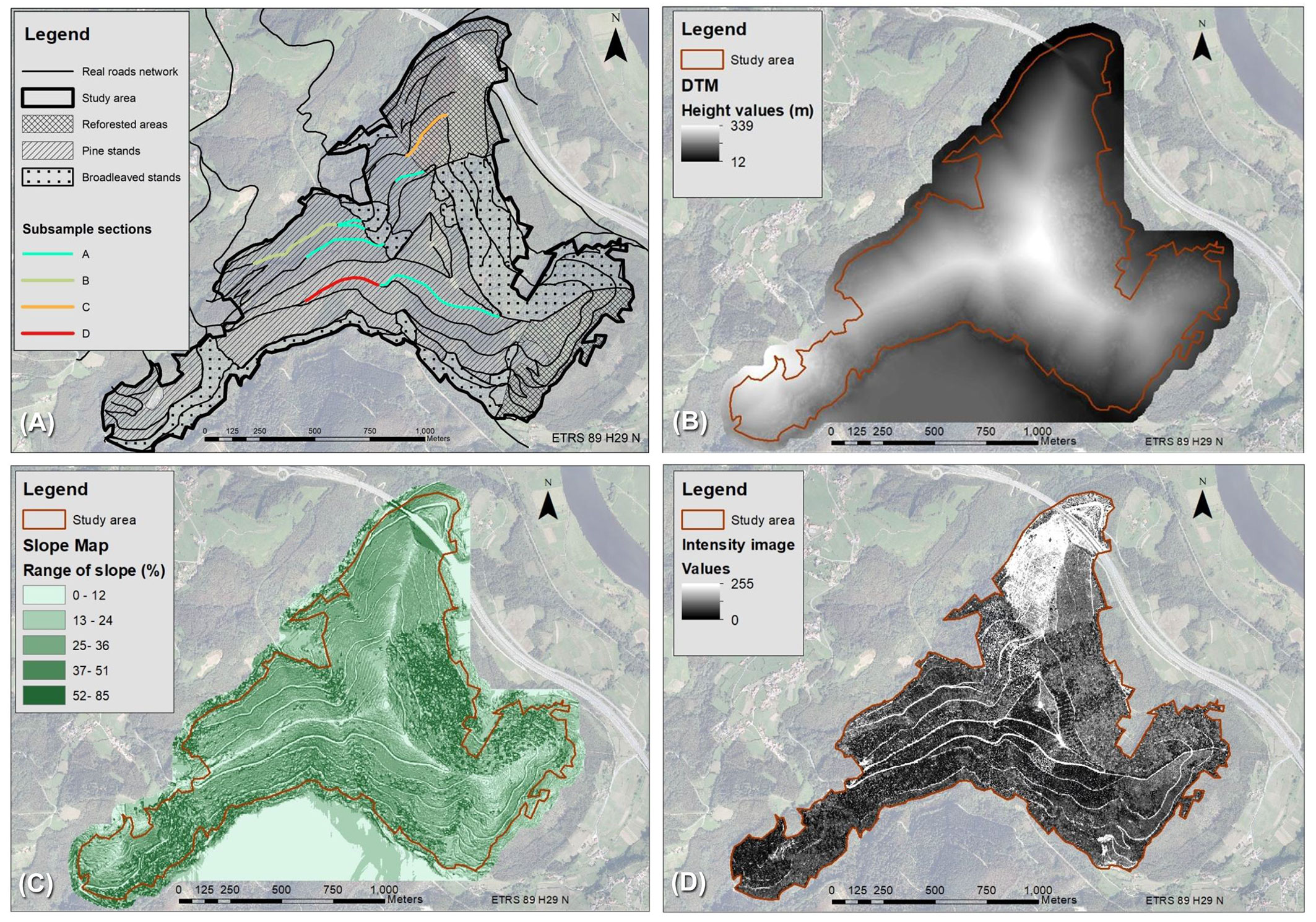
The study area is located in Asturias, a mountainous region situated in the north-west of Spain. A state-owned forest of 178.77 ha was chosen as a pilot area because it is a representative sample of the type of forests found in the region, which are generally characterized by steep slopes and a variety of species. Elevation range is between 36 and 335 meters a.s.l. and over half the area (55.7%) has a slope ranging between 31% and 60%, while 20.7% is above 60%. These characteristics provide a challenging though realistic environment where the detection methodologies of this study could be assessed.
The study area incorporates a number of stand types. There are pure stands of Pinus pinaster Ait. (both mature stands - henceforth: “pine” - and younger reforested areas under 5 years old - henceforth: “reforested”), along with mixed stands of broadleaved species which are dominated by Castanea sativa Mill., but also include Quercus robur L. and Eucalyptus globulus Labill. (henceforth: “broadleaved”). The distribution of the different stand types across the study area is shown in Fig. 1A.
Fig. 1 - (A) Distribution of different stand types across the study area; (B) DTM resulting from the validation step; (C) Slope map resulting from the DTM; (D) Intensity image of the study area.
Data
LiDAR data for the study area was captured under the framework of the PNOA ([29]) during the summer of 2012. Average cloud point density was 0.5 points m-2 and the altimetric accuracy of LiDAR data was around 20 cm.
In order to test the accuracy of the LiDAR detection of forest roads, the real centerlines of the forest roads network in the study area were collected in the field during the summer of 2013 using a GPS Trimble Explorer XH™ (Trimble, Sunnyvale, CA, USA) with submetric accuracy. This data was collected in shape format, whereby the lines defining the centerlines of forest roads are associated with a database which records their main attributes (width and type of road surface and surrounding vegetation).
A further set of field data was also captured using a GPS model with centimetric accuracy (TOPCON GR-3™, TopCon Positioning Systems Inc., Livermore, CA, USA) which was then used to assess the accuracy of the LiDAR-derived products to be used in the analyses. Firstly, to assess the accuracy of the LiDAR-derived DTMs, 55 ground points were measured in the field which were located in areas of varying degrees of slope and different types of vegetation to ensure variability in these factors was covered. Secondly, to evaluate the planimetric accuracy of the LiDAR-derived centerlines obtained with the two approaches, a subsample was selected consisting of four sections of forest roads (A, B, C and D), each with a different type of road surface, and sometimes differing in road width and surrounding vegetation (Tab. 1). The field-survey centerline of each section was digitized for use as a positional reference.
Tab. 1 - Characteristics of the subsample sections.
| Section | Length (m) |
Road surface |
Road width (m) |
Surrounding vegetation |
|---|---|---|---|---|
| A | 994.3 | Aggregate | 2-4 | Pine |
| B | 809.2 | Dirt | 2-4 | Pine |
| C | 266.1 | Rock | 2-4 | Reforested |
| D | 359.8 | Aggregate | >4 | Pine |
LiDAR data processing
For the detection of the forest road network two LiDAR inputs were used: slope map and intensity image. The intensity image enables covered areas to be distinguished from uncovered areas, and the slope map provides information about terrain morphology ([35]).
In order to get an accurate slope map, the first step was to obtain a DTM of the study area. The procedure to obtain a DTM from LiDAR data involves two differentiated steps: the separation of the LiDAR point cloud into those points belonging to the ground and those belonging to tree cover through a filtering process; and the subsequent interpolation of ground points to generate a continuous surface that comprises the DTM. A two-step validation process (see below) was carried out so that the best combination of parameters in each case was established and then used to produce the final DTM.
Filtering quality assessment
Firstly, the filtering of ground points was conducted using the “GroundFilter” function (an adaptation of the IRI filter by Kraus & Pfeifer ([28]) included in the software FUSION ver. 3.5 ([30]). To find the parameters of the “GroundFilter” function (g, w) showing the best performance, 36 combinations were tested in four control areas (each of around 0.5 ha) having specific characteristics making the analysis difficult, such as steep terrain, dense vegetation, etc.). The ranges for each parameter were as follows: g ∈ [-2, -1] at intervals of 0.5 m and w ∈ [1.5, 3.5] at intervals of 1 m. Within the control areas, LiDAR datasets were manually classified as ground and not ground points to obtain a reference dataset for comparison. The validation of the filtering process was carried out following the methodology outlined in Sithole & Vosselman ([36]) and Hu et al. ([25]). The filtering parameters finally selected were g = -1.5 and w = 3.5.
Assessment of LiDAR DTM accuracy
In order to assess the accuracy of the LiDAR DTM, a robust statistical error validation process ([24]) was carried out after generating the candidate DTMs with the various combinations of filter parameters. To do this, the 55 GPS ground captured in the field (see above) were used as control points. All the candidate DTMs had resolution of 2 × 2 m to guarantee that there was at least one point within each pixel.
The DTM which obtained the best results following the two validation steps (Fig. 1B) was selected to generate the slope map (Fig. 1C) which then served as input for the detection approaches.
Due to the fact that intensity values are influenced by terrain, flight and sensor characteristics, as well as by atmospheric conditions ([37]), intensity values need to be corrected. The only data available for this is the average flight height, which can be used to normalize the range, as per the methodology proposed by García et al. ([17]). Based on the normalized intensity values of the LiDAR data, an intensity image was created for a cell size of 2 m (Fig. 1D).
Forest roads detection workflow: pixel-based vs. object-oriented classification (OBIA)
To extract the forest roads from the LiDAR data, the workflow shown in Fig. 2 was followed using two different approaches: a pixel-based classification and an OBIA one. In both cases the intensity image and the slope map were the inputs of the procedure.
Fig. 2 - The workflow followed to obtain LiDAR-derived centerlines.
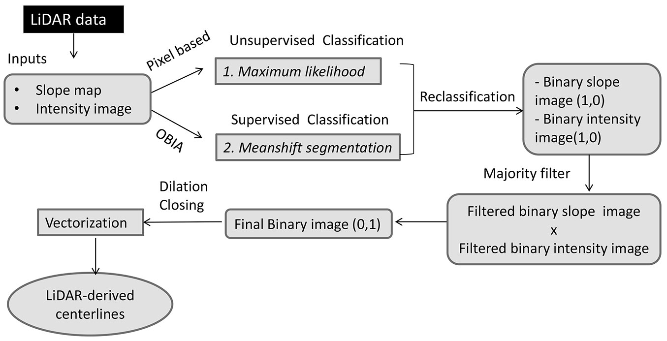
In the first approach, the normalized intensity image and the slope map were subjected to a pixel-level classification using the Maximum Likelihood (ML) algorithm. This method considers that digital levels within each class fit a normal distribution such that each classification category can be described by a probability function deduced from its mean vector and its matrix of variance-covariance. The calculation was performed for all classification categories involved, each pixel being assigned to the category that maximized the probability function ([14]).
In the second approach, the normalized intensity image and the slope map were subjected to an object-oriented unsupervised classification. The algorithm for the segmentation of both images was Meanshift (MS) segmentation ([8]). This algorithm identifies features or segments in an image by grouping together adjacent pixels that have similar spectral characteristics. The amount of spatial and spectral smoothing to assist in the derivation of features of interest can be controlled. Unlike with the ML algorithm, no assumption about probability distributions is made.
The intensity images and slope maps from the two different classification processes used were then reclassified, based on a manual visual analysis, to obtain a binary image - “forest roads” (1) and “not forest roads” (0) - for both slope and intensity.
These binary slope and intensity images were then refined using a majority filter which removes single pixels or noise and replaces the cell(s) depending on the categories of the neighboring cells. After that, the two binary images from each approach were combined by multiplication to obtain one single final binary image, also classified into 0 (not road) or 1 (roads), for the pixel approach and one for the OBIA approach.
This final binary image resulting from each approach was then subjected to a second refining process in order to remove noise and to achieve continuity within category 1 “forest roads” (dilation and closing filter). The final step was automatic vectorization, a technique which converts raster data into vector entities ([31]). Using this technique, a vector file which defined the centerline of the forest roads with a line was obtained (LiDAR-derived centerlines). Visual inspection of these LiDAR-derived centerlines was carried out to ascertain the threshold for noise (established as being 25 m), and all lines not meeting this threshold were removed to reduce noise.
The workflow explained above was automatized with the help of GIS software that uses a Model Builder.
Analysis of results and accuracy assessment
Overall assessment using the quality measures
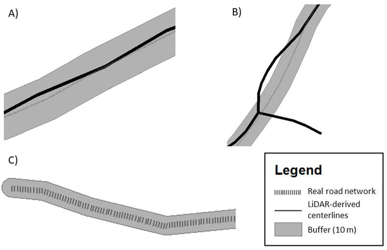
The results from the two approaches were assessed using the methodology described by Azizi et al. ([3]), i.e., the LiDAR-derived centerlines from each approach were compared with the real centerline measured in the field. In order to do this, the real centerline was divided into 500 segments of equal length (48 m) and a 10 meter buffer was built around it (i.e., the area of influence of the forest road). In this way, all LiDAR-derived centerlines located completely within the buffer zone were considered to be detected (“True Positives”, TP - Fig. 3A) and those only partly in the buffer zone were designated as “False positives” (FP - Fig. 3B), while those not identified were classified as “False Negatives” (FN - Fig. 3C)
Fig. 3 - Measures used to calculate the quality measures in forest road detection for the two assessed methodologies. (A) “True Positive” (TP): LiDAR-derived centerlines that are real forest roads. (B) “False Positive” (FP): LiDAR-derived centerlines that do not follow the real road. (C) “False Negative” (FN): forest roads not identified.
From the number of TP, FN and FP found, the quality measures were calculated, as described in the work of Wiedemann et al. ([40]), i.e., completeness (eqn. 1), correctness (eqn. 2) and quality (eqn. 3):
Completeness is the percentage of the reference data (in this case the field data) explained by the extracted data, while correctness represents the percentage of correctly extracted road data. Quality is a more general measure of the final result which combines completeness and correctness into a single measurement. The maximum value for each of the quality measures is 1 (100%).
Influence of the characteristics of forest roads and the surrounding vegetation in the detection
An analysis of variance (ANOVA) was performed to evaluate the influence of various factors on the detection of forest roads, particularly on the quality measures: completeness, correctness and quality. The factors analyzed were: surrounding vegetation type, road surface and road width. All possible combinations of the three factors were considered resulting in a forest road classification of 25 classes. In addition, the influence of the two different approaches used in the detection was also evaluated.
Assessment of accuracy of LiDAR-derived centerlines
Besides estimating the quality of the two methods tested in terms of completeness correctness and quality, the positional accuracy of the centerlines of the LiDAR-derived centerlines was compared to the field-survey centerline of sections A, B, C and D using a simple method proposed by Goodchild & Hunter ([19]). This method is based on the generation of buffers of differing width around the field-survey centerline, after which the percentage of LiDAR-derived centerlines inside each buffer width is calculated. To this end, 20 buffers, at half meter intervals from 0.5 to 10 m were created. Based on the results obtained with the two different approaches, a plot of the percentage of LiDAR-derived centerlines lying within the buffer vs. the buffer width was created and the buffer width required to accommodate 95% of the field-survey centerlines was used as a measure of overall positional accuracy ([19], [38]).
Results and discussion
Overall Assessment of the two approaches (Pixels vs. OBIA)
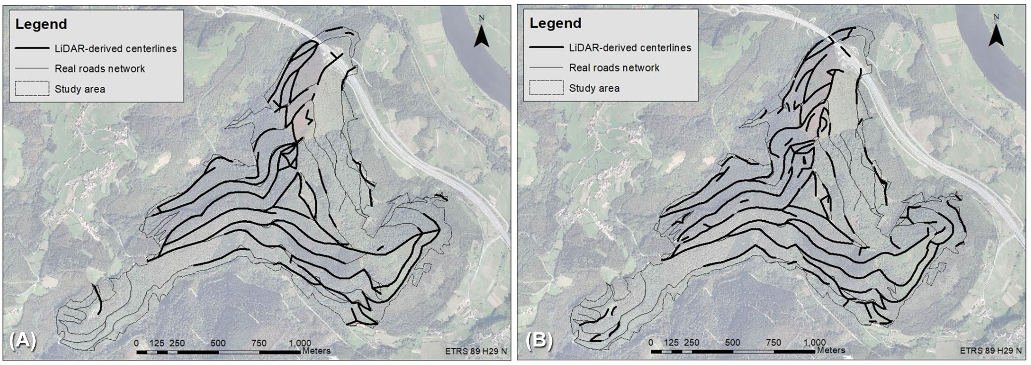
The LiDAR-derived centerlines obtained with each of the two approaches are shown graphically in Fig. 4.
Fig. 4 - Forest road network obtained with the two detection approaches: pixel-based (A) and OBIA (B).
Tab. 2 shows the average values of the quality measures obtained for each of the two approaches assessed in this study.
Tab. 2 - Quality measures obtained for the two detection approaches: pixel-based (Pixels) and OBIA.
| Approach | Completeness | Correctness | Quality |
|---|---|---|---|
| Pixels | 0.65 | 0.90 | 0.60 |
| OBIA | 0.59 | 0.93 | 0.56 |
In terms of completeness, the value obtained in the two approaches was similar, meaning that total percentage of the forest roads network detected with both approaches is around 60-65%. The correctness value was also very similar for both, and indicates that around 90% of the LiDAR-derived centerlines detected automatically represented real roads. Commission error in both cases was therefore low.
Quality provides a more global measure of reliability, since it takes into account both the completeness and the correctness of the extracted data ([41]). The quality value in the pixel-based approach was 4% higher than with OBIA (60 and 56%, respectively). Thus it can be concluded that, as a whole, the pixel-based classification yields slightly better results than the object-oriented one, particularly in terms of quality and completeness.
Influence of the characteristics of forest roads and the surrounding vegetation on detection
Based on the real centerlines collected in the field, the total length of the forest roads network is 24 km, 70% of which were identified in the visual inspection as being in good condition. In relation to road width, the vast majority of forest roads (75%) were wide enough to allow for the circulation of forestry machinery (2.5 m or more).
In this scenario, and despite the heterogeneity of the study area which presented great differences in terms of orography, types of surrounding vegetation and road surface, both approaches were able to detect and draw the centerline of the principal forest roads. Both approaches were particularly effective in areas where road width was > 2.5 m and when roads were not occluded by vegetation, conditions particularly prevalent in the southern part of the study area (Fig. 4A, Fig. 4B).
Tab. 3 reports the results of the ANOVA performed on the quality measures evaluated and shows that there were no statistically significant differences between group averages for the two methodologies used in the detection (Methodology column). However, significant statistical differences were found between all quality measures in the case of vegetation type, and between completeness and quality averages in the case of road width.
Tab. 3 - Results of Analysis of Variance (ANOVA) to quantify the influence of the factors on the quality measures.
| Metric | Vegetation | Road surface | Methodology | Road width | ||||
|---|---|---|---|---|---|---|---|---|
| F | prob | F | prob | F | prob | F | prob | |
| Completeness | 7.92 | 0.0002 | 1.27 | 0.2967 | 0.25 | 0.6205 | 3.97 | 0.0258 |
| Correctness | 6.64 | 0.0008 | 0.98 | 0.4123 | 0.54 | 0.4667 | 2.86 | 0.0677 |
| Quality | 7.49 | 0.0004 | 1.14 | 0.3453 | 0.44 | 0.5120 | 4.8 | 0.0129 |
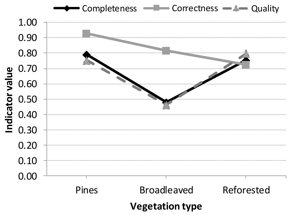
The strongest influence on detection was that of the surrounding vegetation, as can be observed in Fig. 5 which graphically represents the relationship between the values of the quality measures and the surrounding vegetation for the pixel-based classification. It can clearly be observed that all values except correctness are lower for forest roads through broadleaved stands. This suggests that the pixel-based classification works better in areas with wide forest roads which are not surrounded by broadleaved species. Forest road width itself may not be the only factor influencing forest road detection, the width of the belt of forest cleared in order to construct the carriageway is also likely to have a role. However, this is more difficult to quantify with LiDAR technology, and was not taken into account for the purpose of this study. Another issue that should be taken into consideration is the fact that the open space between forest stands due to the forest road and its construction will get smaller over time due to the growth of tree crowns along the stand edge close to the road, which at a certain point may begin to occlude the road itself. In this respect, broadleaved species have globular thick crowns which will generally occupy more space than conifers, and this may have contributed to the lower road detection rates in broadleaved stands.
Fig. 5 - Relationship between the values of the quality measures evaluated in the pixel-based classification and the surrounding vegetation.
Comparing these results with those of other authors, a study carried out by Azizi et al. ([3]) in a forested area using LiDAR data with a density of 4 points m-2 found values of completeness, correctness and quality of 63.02%, 75.07% and 52.17%, respectively. In their case, they used input data (Digital Surface Model and intensity image) from an SVM (Support Vector Machine) classification. The values they found are quite close to those obtained from the pixel-based classification presented here, especially in terms of quality, despite the data used in the present study being of much lower density, only 0.5 points m-2. One reason for this may be that in the work of Azizi et al. ([3]), 80% of its forest roads were under tree cover, which negatively influenced the detection in terms of the low number of ground points resulting in a DTM of 1 meter of resolution. Another study by Sherba et al. ([35]) used a fully automated object-based classification, which performed well with a total accuracy of 86%, a considerable improvement over the pixel-based unsupervised classification used for comparison, which resulted in a road classification accuracy of only 77%. However, it should be taken into account that these authors were working with data of 6 points m-2 and an average road width of 4 meters. In fact they also assessed the influence on the quality of detection of artificially reducing the point cloud density. They found that changing the average point density from 1.2 points m-2 to 0.06 points m-2 resulted in total accuracy falling from close to 70% to below 50%. Determining the optimum data density for forest road detection is challenging, and although all authors agree that the higher the better ([26], [27]), several studies demonstrated that road curves and slope can be assessed from even very sparse (1.12 points m-2) airborne scanning data ([10]). However, in any given area, factors such as road width, type of road surface, surrounding vegetation, etc. will vary, making it difficult to draw definitive conclusions from comparisons between studies.
In the future, in line with the PNOA, when LiDAR data of higher density will be captured for the whole of Spain, the results obtained with the methods detailed in this work will be improved in terms of both quality and positional accuracy. Until such data will be available, the approaches described here can serve to provide the first step in developing a large-scale national database of forest roads networks.
Two limitations of the approaches used here must, however, be recognized. These pertain to forest roads width and the type of vegetation bordering forest roads. The majority of the forest roads that were not detected by either approach are narrow and, on the whole, surrounded by dense broadleaved vegetation. The influence of the type of vegetation is made especially evident by the fact that the centerline of forest roads running through broadleaved stands is at times completely occluded, thus making road detection exceedingly difficult. It should be noted that the LiDAR data used in this study was captured during summer, when broadleaved canopies were in full leaf. Thus, the laser beam cannot penetrate through the dense canopy to the ground, resulting in a lower quality DTM not representing the shape of the land surface, but rather of the vegetation. In the case of intensity image, the leafy areas appear very dark because they represent the highest points of the vegetation, especially in those areas where the high canopy density hinders the centerline of a forest road to be detected from the air, or is completely masked. In areas where there are two types of vegetation stand adjacent to each other, such as pine and broadleaved stands, it can be seen that the LiDAR-derived centerline was detected without problem in the pine forest area but disappears or is interrupted in the part bordered by broadleaved trees.
In reforested stands however, the percentage of LiDAR-derived centerlines detected was high, since the relatively recently planted vegetation was not very dense and did not occlude the centerlines of the roads. However, the number of false positives in these areas was also high, because the presence of bare soil among the trees gives rise to high intensity values, and the classification algorithm has problems distinguishing soil between lines of smaller young trees from the surface of the road. According to the results of Beck et al. ([4]), differences in canopy cover proved to be a weakness in the road extraction process, which requires relative consistency of cover type to define intensity thresholds. Extreme differences in cover type throughout an area will have a large impact on results of the road extraction process. False positives in particular are more sensitive to these differences.
In this study, forest roads that did not have pronounced gradient were difficult to identify, as can be observed in the bottom left corners of Fig. 4A and Fig. 4B where slope is around 20%. This has also been documented by White et al. ([39]) and Azizi et al. ([3]). Areas of gentle gradient can also cause breaks in the continuity of the forest roads network when drawing the centerline ([15]).
Assessment of positional accuracy of LiDAR-derived centerlines
The results of the assessment of the positional accuracy of the LiDAR-derived centerlines obtained with the method of Goodchild & Hunter ([19]) are shown in Fig. 6, which plots the percentage of the LiDAR-derived centerline lying within the buffer against buffer width for each approach, pixel-based (6A) and OBIA (6B).
Fig. 6 - Percentage of LiDAR-derived centerline lying within the buffer as a function of buffer width using pixel-based approach (A) and OBIA approach (B).
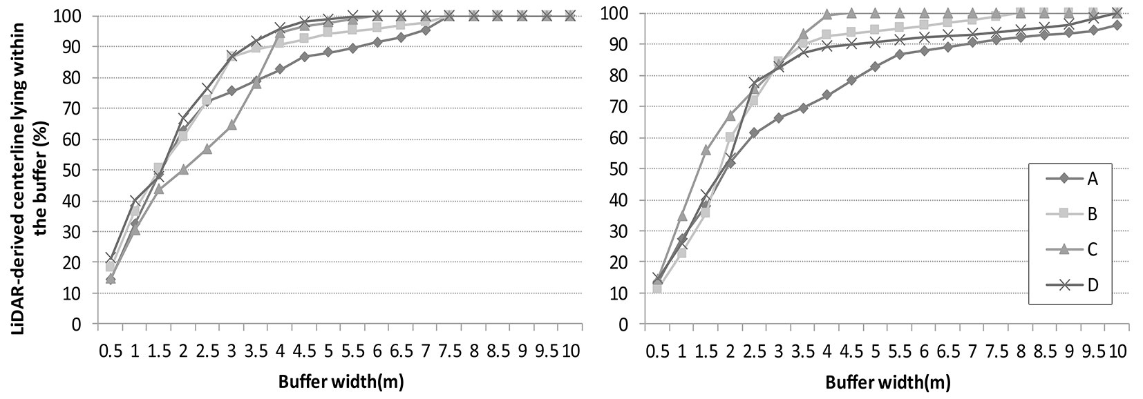
Tab. 4 shows the positional accuracy of each approach in each of the sections examined, that is, the width of the buffer needed to encompass 95% of the field-survey centerline. In general, the pixel-based classification gave better results, especially in section D, where the accuracy difference between the two approaches was 4 m. The higher accuracy in this section is due to the combination of two most favorable factors, big width (more than 4 m) and surrounding vegetation composed by pines which was the kind of stand having the best behavior in terms of forest roads detection.
Tab. 4 - Positional accuracy values (in meters) for the two approaches for each section.
| Section | Length (m) |
Road surface |
Road width (m) |
Vegetation | Pixel | OBIA |
|---|---|---|---|---|---|---|
| A | 994.3 | Aggregate | 2-4 | Pine | 7.00 | 10.00 |
| B | 809.2 | Dirt | 2-4 | Pine | 5.50 | 5.50 |
The average positional error was ± 5.50 m for the pixel-based approach and ± 6.88 for OBIA. In the case of LiDAR-derived centerline accuracy, the fact that the pixel-based classification was more accurate may be related to the resolution of the images used in the classification process. According to Cánovas-García ([6]), the object-oriented classification approach is capable of delivering more accurate results than those obtained by a pixel-based approach, especially when dealing with high spatial resolution images. However, in this case the resolution of the information layers involved in the detection of forest roads was not high because of the low density of the data used, and this may have counteracted the difference found by Cánovas-García ([6]). In addition, Cowen et al. ([9]) highlight the fact that the object to be identified must be composed of at least 4 pixels if remote sensor images are used, a condition which was not always met in this study. As a result, the advantage of OBIA methods over pixel-based methods, that is the ability to generalize and reduce heterogeneity, becomes a drawback with low density data. Finally, much of the study area has a high degree of slope and dense vegetation which, together with the narrower width of some of the forest roads and the low resolution of the information layers, makes it difficult to create objects that are representative of roads in the segmentation process.
Comparing the results obtained in this study with other similar works, accuracy values are lower than those obtained by White et al. ([39]) and Azizi et al. ([3]) (1.3 and 1.2 m respectively). This may be due in large part to the low density of the LiDAR data used in this study (0.5 points m-2 vs. 12 and 4 points m-2, respectively) which forces the slope map and the intensity image to have a low resolution compared to the images used in the abovementioned papers. Morever, forest roads width in both these studies is, on average, greater than that in this study. In the case of White et al. ([39]), the process of digitizing the centerline was manual, while in this study it was completely automatic. Although this introduces a certain degree of error, it has the great advantage that it can be applied to large areas at very low cost. For example, Gao & Wu ([16]) report that the automatic extraction of road network information involves significantly less time and expense, though it is methodologically more complex. Doucette et al. ([13]) defines productivity in relation to digitization of data as being the time taken to digitize the information per measure of area. Roman et al. ([33]) in an area with similar characteristics to those of this study, found manual digitization to have a productivity of 1 km per minute. In contrast, the productivity of the semi-automatic process presented here is 1 km in 9.2s (using a computer with 8 GB of RAM). Based on these data, the use of the proposed method allows productivity to be increased more than 6 fold with respect to the manual method. Moreover, the positional accuracy of ± 5.50 m obtained here is still much better than the ± 12 m obtained by USGS (United States Geological Survey) in their topographic maps, or the ± 10 m used in traditional data sources to plot roads on the 1:25.000 topographic maps in Iran ([3]). It is also very similar to the ± 5 m positional accuracy of the mapping of the Spanish public road network, demonstrating that even the low density data used in this work can provide estimations as good as, and often better than, existing cartographies.
One final point to note is that forestry road extraction is typically a manual process where positional error depends on a number of factors, but the human factor (i.e., differences depending on the person making the digitization) has been reported to be approximately 3 meters ([13]). As such, one of the main advantages of automatic vectorization techniques is that the effect of the individual disappears, and hence accuracy error depends only on the data sources and the vectorization methodology. Finally, if mapping were conducted over larger extents (hundreds to thousands of square kilometers) automated and semi-automated road extraction techniques could offer substantial savings in terms of time ([13]).
Conclusions
In this study a methodology for the detection and extraction of forest roads from freely available LiDAR data of low density was designed and applied. The results obtained confirm the initial hypothesis that it is possible to semi-automatically reconstruct the forest roads network even in steep forested environments. As the analysis procedure has been implemented in a GIS Model Builder, it can be applied quickly and easily in other forest areas with similar or less complex and challenging characteristics.
Of the two approaches evaluated, the pixel-based classification method yielded slightly better results than the OBIA one with regard to the quality measures and positional accuracy. The completeness, correctness, and quality values were 65%, 90% and 60%, respectively, compared to 59%, 93% and 56% obtained with OBIA. Despite this, the results of the ANOVA demonstrate that neither the methodology used nor the type of road surface had any significant influence on the detection and digitization of the road centerline, although road width and the type of surrounding vegetation do. In fact, the results indicate that low density LiDAR data is suitable for the detection and digitization of forest roads over large areas, especially those where forest roads are wider (over 4 m) and are not surrounded by broadleaved stands. With respect to positional accuracy, the values obtained by pixel-based classification are on average, 1.38 m more accurate than those from the OBIA for each of the sections examined (± 5.50 vs. ± 6.88 m, respectively). The value of ± 5.50 m can be considered acceptable given that traditional data sources used to plot roads have lower accuracy values than this.
Regarding the methodology limitations, future research should focus on both improving the effectiveness of image classification and achieving more defined and continuous lines (road centerlines) in adverse vegetation and slope conditions.
Finally, efforts at a national level by governments to capture higher cloud point density data on a country-wide level open the door to large-scale detection trials. In Spain, the data that will be captured in the future, within the framework of PNOA, will allow the methodology presented in this study to be used to develop a cartography of forest roads, including mountainous areas, which can be updated every time new data is released. However, in the meantime, the approaches described in this work offer a valuable first step towards such a complete large-scale database of forest roads networks.
Acknowledgements
This study was funded by the SCALyFOR project (R&D Projects “Research Challenges”, Spanish Ministry of Economy and Competitiveness). The authors would like to thank the Forestry Service of the Principality of Asturias (Spain) for providing the information used. Thanks also to Ronnie Lendrum for revising the English.
References
Online | Gscholar
Gscholar
Gscholar
CrossRef | Gscholar
CrossRef | Gscholar
Gscholar
Gscholar
Authors’ Info
Authors’ Affiliation
Elena Canga 0000-0003-2132-9991
CETEMAS, Centro Tecnológico y Forestal de la Madera, Área de Desarrollo Forestal Sostenible. Pumarabule, Carbayín Bajo s/n 33936 Siero (Spain)
Laboratorio do Territorio (LaboraTe), Universidad de Santiago de Compostela. C/ Benigno Ledo Campus Universitario 27002 Lugo (Spain)
Departamento de Explotación de Minas, Grupo de Investigación en Geomática y Computación Gráfica (GEOGRAPH), Universidad de Oviedo, 33004 Oviedo (Spain)
Corresponding author
Paper Info
Citation
Prendes C, Buján S, Ordoñez C, Canga E (2019). Large scale semi-automatic detection of forest roads from low density LiDAR data on steep terrain in Northern Spain. iForest 12: 366-374. - doi: 10.3832/ifor2989-012
Academic Editor
Agostino Ferrara
Paper history
Received: Nov 05, 2018
Accepted: Apr 15, 2019
First online: Jul 05, 2019
Publication Date: Aug 31, 2019
Publication Time: 2.70 months
Copyright Information
© SISEF - The Italian Society of Silviculture and Forest Ecology 2019
Open Access
This article is distributed under the terms of the Creative Commons Attribution-Non Commercial 4.0 International (https://creativecommons.org/licenses/by-nc/4.0/), which permits unrestricted use, distribution, and reproduction in any medium, provided you give appropriate credit to the original author(s) and the source, provide a link to the Creative Commons license, and indicate if changes were made.

Web Metrics
Breakdown by View Type
Article Usage
Total Article Views: 34619
(from publication date up to now)
Breakdown by View Type
HTML Page Views: 29197
Abstract Page Views: 2139
PDF Downloads: 2795
Citation/Reference Downloads: 3
XML Downloads: 485
Web Metrics
Days since publication: 1750
Overall contacts: 34619
Avg. contacts per week: 138.48
Article Citations
Article citations are based on data periodically collected from the Clarivate Web of Science web site
(last update: Feb 2023)
Total number of cites (since 2019): 10
Average cites per year: 2.00
Publication Metrics
by Dimensions ©
Articles citing this article
List of the papers citing this article based on CrossRef Cited-by.
Related Contents
iForest Similar Articles
Technical Reports
Qualitative evaluation and optimization of forest road network to minimize total costs and environmental impacts
vol. 5, pp. 121-125 (online: 05 June 2012)
Technical Reports
Decision making in forest road planning considering both skidding and road costs: a case study in the Hyrcanian Forest in Iran
vol. 6, pp. 59-64 (online: 21 January 2013)
Research Articles
Evaluation of urban forest landscape health: a case study of the Nanguo Peach Garden, China
vol. 13, pp. 175-184 (online: 02 May 2020)
Research Articles
Accuracy assessment of different photogrammetric software for processing data from low-cost UAV platforms in forest conditions
vol. 12, pp. 435-441 (online: 01 September 2019)
Research Articles
Application of indicators network analysis to support local forest management plan development: a case study in Molise, Italy
vol. 5, pp. 31-37 (online: 27 February 2012)
Editorials
Adaptation of forest landscape to environmental changes
vol. 2, pp. 127 (online: 30 July 2009)
Research Articles
How do urban dwellers react to potential landscape changes in recreation areas? A case study with particular focus on the introduction of dendromass in the Hamburg Metropolitan Region
vol. 7, pp. 423-433 (online: 19 May 2014)
Short Communications
The Polish landscape changing due to forest policy and forest management
vol. 2, pp. 140-142 (online: 30 July 2009)
Research Articles
Use of LIDAR-based digital terrain model and single tree segmentation data for optimal forest skid trail network
vol. 8, pp. 661-667 (online: 22 December 2014)
Research Articles
Examining the evolution and convergence of wood modification and environmental impact assessment in research
vol. 10, pp. 879-885 (online: 06 November 2017)
iForest Database Search
Search By Author
Search By Keyword
Google Scholar Search
Citing Articles
Search By Author
Search By Keywords
PubMed Search
Search By Author
Search By Keyword


