Effect of imperfect detection on the estimation of niche overlap between two forest dormice
iForest - Biogeosciences and Forestry, Volume 11, Issue 4, Pages 482-490 (2018)
doi: https://doi.org/10.3832/ifor2738-011
Published: Jul 18, 2018 - Copyright © 2018 SISEF
Research Articles
Abstract
Quantification of niche overlap represents an important topic in several aspects of ecology and conservation biology, although it could be potentially affected by imperfect detection, i.e., failure to detect a species at occupied sites. We investigate the effect of imperfect detection on niche overlap quantification in two arboreal rodents, the edible dormouse (Glis glis) and the hazel dormouse (Muscardinus avellanarius). For both species, we used Generalized Linear Mixed Models (GLMM) to estimate the occurrence probability and Occupancy Models (OM) to calculate occurrence and detection probabilities. By comparing these predictions through niche equivalency and similarity tests, we first hypothesised that methods correcting for imperfect detection (OM) provide a more reliable estimate of niche overlap than traditional presence/ absence methods (GLMM). Furthermore, we hypothesised that GLMM mainly estimate species detectability rather than actual occurrence, and that a low number of sampling replicates provokes an underestimation of species niche by GLMM. Our results highlighted that GLMM-based niche overlap yielded significant outcomes only for the equivalency test, while OM-based niche overlap reported significant outcomes for both niche equivalency and similarity tests. Moreover, GLMM occurrence probabilities and OM detectabilities were not statistically different. Lastly, GLMM predictions based on single sampling replicates were statistically different from the average occurrence probability predicted by GLMM over all replicates. We emphasized how accounting for imperfect detection can improve the statistical significance and interpretability of niche overlap estimates based on occurrence data. Under a habitat management perspective, an accurate quantification of niche overlap may provide useful information to assess the effects of different management practices on species occurrence.
Keywords
Occupancy Models, Generalized Linear Mixed Models, Forest Management, Niche Overlap
Introduction
The niche is a central concept in ecology and evolution that dates back at least to Grinnell ([26]). The fundamental ecological niche as conceptualized by Hutchinson ([29]) is the space bounded by an n-dimensional hypervolume, consisting of a range of abiotic and biotic variables, wherein a species is able to persist indefinitely in the absence of competition.
Concerns on how global change will influence niche dynamics in evolutionary and community contexts, highlight the growing need for robust methods to quantify niche differences between or within taxa ([11]). During the last decade, statistical approaches have been developed allowing to compare species niches in a gridded environmental space ([53], [11]). As a consequence, the estimation of niche overlap has become an important tool for investigating ecological requirements of invasive species ([25]), relative abundance distributions ([38]), species coexistence ([25]), evolutionary diversification ([2]) and conservation strategies ([48]). However, specific factors were shown to affect estimates of niche overlap. For instance, recent studies highlighted how niche overlap quantification may yield misleading results depending on the grain size ([32]) and the geographical scale ([48]) used to perform the analysis. Among other factors, imperfect detection, i.e., failure to detect a species at occupied sites was shown to affect niche estimation itself. For instance, predictions of species distribution through species distribution modelling (SDM), which are based on quantifying realized niche by means of the spatial (geographic) distribution of species across a study area ([46]), may be underestimated if not accounting for imperfect detection ([47], [33]). In light of this evidence, investigating which bias could be introduced when quantifying overlap of two niches that are already affected by imperfect detection, represents an intriguing research topic.
Niche estimation and modelling typically relies on presence/absence or presence/ background data ([33]). However, these data could be biased by the fact that species (both animals and plants - [17]) often remain undetected, making imperfect detection a serious issue in species surveys ([33], [27]), and a major source of bias in wildlife distribution studies ([35]). Unless a suitably large sampling effort is invested at surveyed locations, imperfect detection will result in the recording of false absences in presence/absence data, potentially leading to biased conclusions and incorrect conservation actions ([35], [24]). Many studies demonstrated that detectability varies among species, over time, and among habitats, and there may be serious consequences when this variability is ignored ([27]). The occurrence of a species could be easy to prove, but species absence and non-detection can be often confounded, especially in case of species with low detectability ([35], [36]).
A popular approach was proposed to overcome this problem by explicitly accounting for imperfect detection when quantifying species distribution ([36], [3]). Hence, the so-called “occupancy models” are based on the detection history at sites and the proportion of sites where the species is detected, jointly modelling the processes describing where the species occurs and its detection at occupied sites ([35]). In recent years, several studies highlighted the importance of explicitly accounting for imperfect detection when modelling species distribution ([47], [33]), though its effect on the quantification of niche overlap among species have been surprisingly overlooked. We aimed at filling this gap by evaluating the effect of imperfect detection on the quantification of niche overlap between two sympatric forest rodents. Specifically, we aimed at testing the following hypotheses:
- H1: the probability of occurrence corrected for imperfect detection provides a more reliable estimate of niche overlap than predictions from traditional presence/absence methods;
- H2: predictions of occurrence probability derived from traditional presence/absence methods reflects the species detectability rather than its actual occurrence pattern;
- H3: a low number of sampling replicates in traditional presence/absence methods causes an underestimation of species niche.
The three hypotheses respectively focused on niche overlap between species (H1), between modelling methods (H2) and among sampling replicates (H3). We targeted the analyses to two arboreal rodents: the edible dormouse (Glis glis) and the hazel dormouse (Muscardinus avellanarius), occurring sympatrically in a Central Apennines deciduous forest.
Although both species are strictly forest dependent, they exhibited different ecological preferences with regard of forest characteristics ([15], [44]) therefore representing ideal candidate species for a niche comparison study. The two species were surveyed with a sampling design addressed to provide both occurrence and detection probabilities ([35]). Fine scale environmental covariates were then measured at each sampled plot and related to both occurrence and detectability.
Materials and methods
Study area
The study area is located in Central Apennines (Molise, Italy; 41° 43′ N, 14° 06′ E - Fig. 1), with an elevation ranging from 650 to 1300 m a.s.l.
Fig. 1 - Map of the study area with sampling plots location.
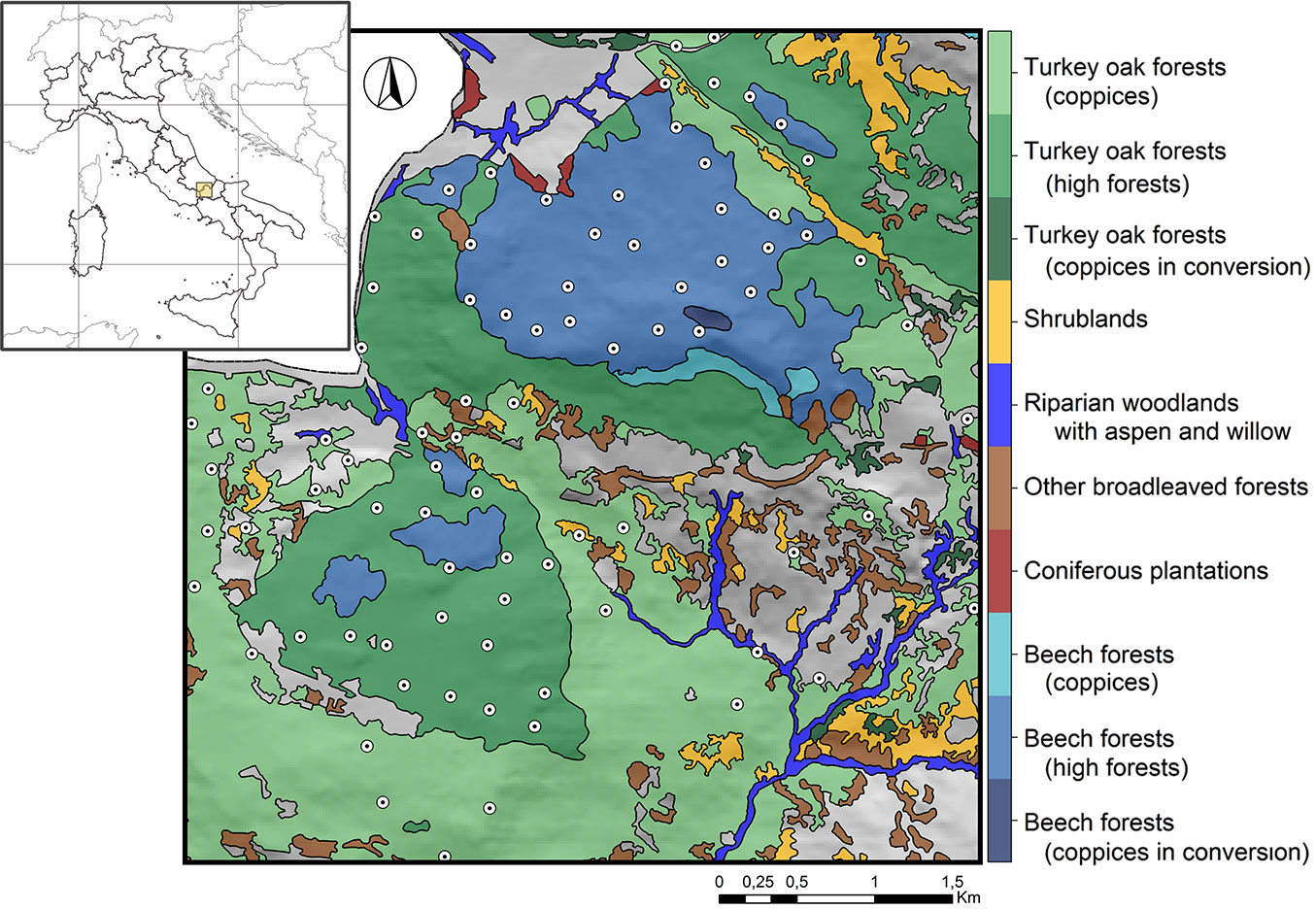
The area covers approximately 18 km2 and it is mainly dominated by European beech (Fagus sylvatica L.) and Turkey oak (Quercus cerris L.) forests ([52]), with different ownership, forest structures (i.e., coppices and high forests) and management objectives (i.e., timber harvesting, biodiversity conservation, hydrogeological protection etc.). The climate is classified as “temperate”, with a mean annual precipitation of 1100 mm and a mean annual temperature of 8.6 °C ([7]).
According to Amori et al. ([1]), the study area hosts 25 small mammal species, including 14 rodents (order Rodentia, families Cricetidae, Gliridae, Muridae and Sciuridae) and 11 insectivores (order Eulipotyphla, families Erinaceidae, Soricidae and Talpidae), most of which (ca. 58%) are listed in the Appendix III of the Bern Convention, in the Annex IV of 357/97/EC Habitats Directive or are protected by the Italian law 157/1992.
Dormice occurrence sampling
A total of 83 sampling plots were randomly located in the study area with a minimum distance of 200 m (mean nearest neighbour distance = 316 ± 111 m), in order to guarantee the independence of data based on the average home range size of the target species ([8], [9], [39]). A nest box and a hair-tube were installed at each site (see Appendix 1 in Supplementary material). Sampling plots were checked for species presence/absence at 15 days intervals during the pre-hibernation period from the end of August until mid-October 2013 ([44], [1]) for a total of four sampling replicates. Specifically, nest boxes were considered occupied either when individuals, nests, food remains or droppings were detected inside the box ([10]). Species presence at hair-tubes was determined by analysing hair samples found inside the tubes (for further details on the hair identification protocol, see Appendix 1 in Supplementary material).
Forest parameters estimation and selection
A set of 12 dendrometric and typological-structural forest parameters were measured at each sampling plot following the Italian National Forest Inventory protocol ([23] - see also Appendix 2). In particular, dendrometric attributes were measured for all the living trees with a Diameter at Breast Height (DBH) ≥ 7.5 cm, considering circular plots of 13 m radius. Forest attributes related to deadwood were also quantified within the same circular plots ([34]). Typological-structural parameters including forest category, forest management and stand age were attributed according to the regional forest type and age maps ([52], [22]). Numerical covariates were standardized and sub-selected to avoid multicollinearity, considering a Variance Inflation Factor lower or equal to 10 ([54]). This procedure led to a final set of seven forest predictors that were included in the subsequent analyses (Tab. 1).
Tab. 1 - Explanatory variables used for GLMM and OM.
| Forest parameter | Type | Levels | Description |
|---|---|---|---|
| Forest category (F_cat) | Categorical | Beech forest | Category of forest defined by its composition |
| Turkey oak forest | |||
| Forest management (F_man) | Categorical | Coppice with standard | Prevalent silvicultural system adopted |
| Coppice in conversion to high forest | |||
| Mature high forest | |||
| Tree species richness (SR) | Continuous | - | Number of tree species (n) |
| Tree density (T_density) | Continuous | - | Mean number of trees per hectare (n ha-1) |
| Mean of the trees’ heights (Mean_height) | Continuous | - | Average height of trees (m) |
| σ² Height (Stdev_height) | Continuous | - | Standard deviation of trees heights (m) |
| Stand basal area (Basal_area) | Continuous | - | The cross-sectional area of the tree stems measured at breast height (m2 ha-1) |
Modelling framework
The modelling framework proceeds through three steps: (1) investigate the statistical relationships between species presence/absence and forest covariates through Generalized Linear Mixed Models (GLMM) and Occupancy Models (OM); (2) calculate the niche overlap between the two target species starting from the values of occurrence probability predicted by both modelling approaches; (3) quantify, for both species, the degree of niche similarity between GLMM and occupancy predictions, and by GLMM and detectability predictions, respectively.
Generalized linear mixed models
To investigate the statistical relationship between species occurrence and forest variables, we applied GLMM ([37]) implemented in the “lme4” package ([5]) of R statistical language ver. 3.4.0 ([45]). GLMM proved useful when repeated measurements are made on the same statistical units (i.e., longitudinal studies), therefore violating the independence of sampling units ([55], [30]). The presence/absence data detected at each site during the four sampling replicates were used as response variable. We started from a full model including, as fixed effect terms, all the seven forest covariates (allowing both linear and quadratic relationships for the continuous ones), along with an interaction term with forest management (Tab. 1). Besides, we considered the sampling replicate as random effect. Specifically, we allowed the model to change its intercept according to the sampling replicate to take into account non-independence of data between different sampling of the same sites. We then applied a variable selection procedure allowing to compare models with all the possible combinations of the starting covariates and random effect terms. The “dredge” function in the R package “MuMIn” ([4]) was used for model selection, ranking the candidate models according to their AICc ([13]). To account for uncertainty in model selection, we used a model averaging approach (i.e., we averaged all models within two ΔAICc of the top model - [14], [42]). The goodness-of-fit of the models was assessed by calculating the conditional and marginal coefficients of determination for GLMM (R_GLMM2 - [43]).
Conditional R_GLMM2 is interpreted as the variance explained by both fixed and random factors (i.e., the entire model), whereas marginal R_GLMM2 refers to variance explained by the fixed factors (i.e., excluding the random effect - [43]).
Occupancy models
This statistical approach consists of two hierarchically coupled sub-models, one governing the true state of sites (presence/ absence) and the other governing the observations (detection/non-detection - [35]). OM can correct for imperfect detection due to false absences (i.e., failure to detect a species that is present at the site - [35]), which represents a major source of bias in wildlife distribution studies ([35], [36]). We applied a single-season, single-species model ([35]) to compute the probability of occurrence (occupancy, ψ) and the probability of detecting the species (detectability, p), using the R package “unmarked” ([21]). In this case, we used the detection history of each species per site, i.e., the sequence of presences/absences over the complete survey period (four replicates), as response variable in the model. Similarly to GLMM, we started from a full model including all the seven forest covariates (allowing both linear and quadratic relationships for the continuous ones), along with an interaction term with forest management. Following Mortelliti et al. ([40]), we split the variable selection procedure in two steps: (1) the detection probability was modelled as a function of different combinations of forest predictors, keeping the occupancy as constant and retaining the best subset of variables in the subsequent step; (2) the selection procedure was repeated simultaneously including both occupancy and detectability, while including, for the latter, only the variables combinations selected in step 1. As for GLMM, we averaged all models within ΔAICc ≤ 2 from the top model. The goodness-of-fit of each model was measured using the Nagelkerke’s pseudo-R2 ([41]). Predicted values of occurrence probability (from GLMM), ψ and p (from OM) were projected over the study area by spatializing the predictors selected in the top-ranked models (i.e., models within ΔAICc ≤ 2). Further details on the spatialization procedure are provided in Appendix 3 (Supplementary material).
Niche overlap
For both species, we ran the niche overlap analyses considering the following parameters: Pocc_ (average values of occurrence probability predicted by GLMM along all of the four replicates), Pocc_rep_i_ (occurrence probability predicted by GLMM for the i-th sampling replicate); Psi_ (occurrence probability predicted by OM), Det_ (detection probability predicted by OM). The flowchart of the methodological sequence followed to implement niche overlap analyses is depicted in Fig. 2.
Fig. 2 - Flowchart of the niche overlap analysis implemented to test the three study hypotheses. White rectangles with black borders refer to occurrence probability values predicted by GLMM, grey rectangles with rounded borders indicate occupancy values predicted by OM and grey rectangles with squared borders indicate detectability values predicted by OM. Dashed arrows refer to niche equivalency and similarity tests used to compare the predictions.
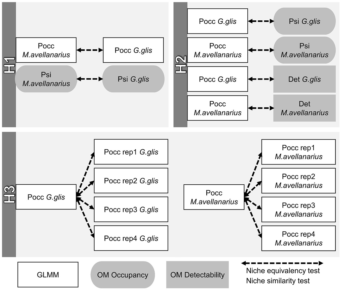
To test H1, we performed the following niche overlap tests: Pocc_Gglis vs. Pocc_Mavellanarius and Psi_Gglis vs. Psi_Mavellanarius. Then, we compared Pocc_ vs. Psi_and Pocc_ vs. Det_for both species to test H2. Lastly, we tested H3 by calculating Pocc_ vs. Pocc_rep_i_, for both species and the four sampling replicates, separately. All the niche overlap tests are shown in Fig. 2.
Analysis of niche overlap between the two species was carried out using the analytical framework proposed by Broennimann et al. ([11]) and recently adopted in different studies ([48]). Within this framework, the environmental space is defined by the axis of occurrence probabilities predicted by GLMM and OM for the two species. The output of such models comprises a single vector of predicted occurrence probabilities derived from complex combinations of functions of original environmental variables; the niche overlap is analysed along this gradient of predictions ([11]). Niche overlap was computed in terms of Schoener’s D ([49]), a metric that ranges from 0 (no overlap) to 1 (complete overlap).
We performed niche equivalency and similarity tests sensu Warren et al. ([53]). The first test evaluates if the two species are identical (null hypothesis) in their niche space by using their exact locations and not including the surrounding space. The second also accounts for the differences in the surrounding environmental conditions and assess if the two species are more different than expected by chance. In particular, similarity between niches was tested in both directions, i.e., the amount of species 1 niche included in species 2 niche, and vice versa, following Broennimann et al. ([11]). All the procedures were performed using the R package “ecospat” ([12]).
Results
Throughout the duration of the study, we reported 31 detections of G. glis at 27 of 83 sampling plots and 31 detections of M. avellanarius at 16 of 83 sampling plots (further details are provided in Tab. S1, Supplementary material). In GLMM, model selection procedure identified 15 top-ranked models for G. glis and three for M. avellanarius out of 3136 candidate models. Both species showed high values of conditional R_GLMM2 (G. glis: mean = 0.523, SD = 0.065; M. avellanarius: mean = 0.640, SD = 0.006). Conditional R_GLMM2 were always higher than marginal ones, indicating that the inclusion of the random effect systematically improved the models goodness-of-fit (Tab. S2). Occurrence of G. glis was predominantly explained by stand basal area (15 models) through a direct relationship. In addition, eight out of 15 top-ranked models predicted higher occurrence probabilities at increasing tree density values and in Turkey oak stands (Tab. S2, Fig. 3b). For M. avellanarius, mean tree height and interaction between tree density and forest management were the most important variables, resulting inversely related with species occurrence in all the top-ranked models. In addition, standard deviation of tree height and forest category were retained in more than a half of the top-ranked models, predicting higher occurrence probabilities in forests with high variability in tree heights and beech stands (Tab. S2, Fig. 3c).
Fig. 3 - Models’ outcomes. The two rows show results for GLMM and OM, respectively. First column depicts niches of edible (dark grey) and hazel (light grey) dormice calculated from GLMM (a) and OM (d) predictions. Yellow areas refer to niche overlap. Circles (a, d) show the significant outcomes (white) of the equivalency and similarity tests. Bar plots on the right display variables importance for the two species calculated by GLMM (b, c) and OM (e, f), as the cumulative sum of Akaike weights over the top-ranked models. Only variables being selected in at least a half of the top-ranked models were included. For forest management (F_man) two of the three levels are shown: high forests (dark grey) and coppices in transition (black). For forest category (F_cat) the level referring to “Turkey oak” category was displayed.
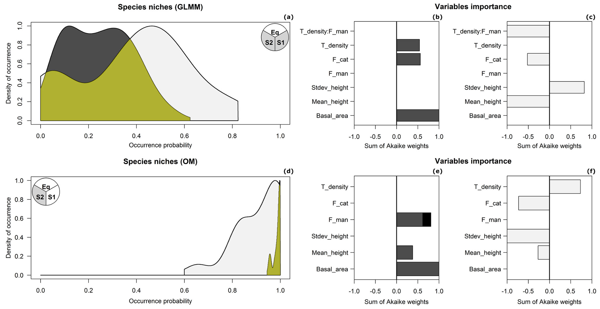
In OM, the final model set included eight top-ranked models for G. glis and two for M. avellanarius out of 3136 candidate models. Goodness-of-fit statistics for the top-ranked models reported a mean pseudo-R2 equal to 0.370 (SD = 0.033) for G. glis and to 0.549 (SD = 0.030) for M. avellanarius (Tab. S3 in Supplementary material). For G. glis, both occupancy and detectability were directly related with stand basal area in all the top-ranked models. Six out of eight models also included forest management, predicting higher occupancy values in high forests and coppices in conversion rather than in coppices. Besides, mean tree height was retained in four models, always showing a direct relationship with the occurrence probability (ψ - Tab. S3, Fig. 3e). For M. avellanarius, occupancy was predominantly explained by standard deviation of tree heights, showing an inverse relationship in both top-ranked models. In addition, tree density and forest category were retained in half of the top-ranked models, predicting higher occupancy values in dense forests and beech stands (Tab. S3, Fig. 3f). Finally, M. avellanarius detectability was mainly explained by mean and standard deviation of tree height and tree density (Tab. S3 in Supplementary material). Maps of predicted detectability for the two species show overall higher values of p for M. avellanarius (mean = 0.192, SD = 0.041) than for G. glis (mean = 0.154, SD = 0.004; Fig. 4). For both species, GLMM predicted lower values of occurrence probability (G. glis: mean = 0.104, SD = 0.083; M. avellanarius: mean = 0.114, SD = 0.201) than probability values corrected by detectability under OM (ψ, G. glis: mean = 0.599, SD = 0.163; M. avellanarius: mean = 0.504, SD = 0.337 - Fig. S1).
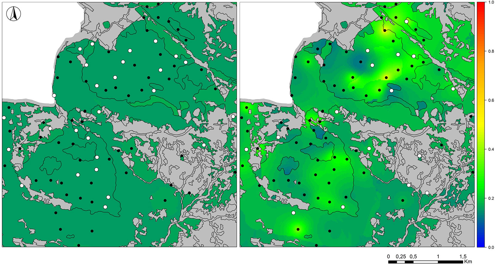
Fig. 4 - Maps of predicted detection probabilities for G. glis (left) and M. avellanarius (right). Detectability values, which range from 0 (blue) to 1 (red), were projected over the study area by spatializing the predictors selected in the top-ranked models (see also Appendix 3 in Supplementary material). White (black) dots indicate presence (absence) sites.
As for niche overlap tests, GLMM’s Pocc_Gglis vs. Pocc_Mavellanarius (Schoener’s D = 0.41 - Fig. 3a) showed significant outcomes only for the equivalency test. On the other hand, niche overlap computed on OM’s Psi_Gglis vs. Psi_Mavellanarius (Schoener’s D = 0.26 - Fig. 3d) yielded significant outcomes for both niche equivalency and similarity (i.e., niche 1 vs. niche 2 - Fig. 3a, Fig. 3d, Tab. 2).
Tab. 2 - Results of niche overlap tests. (Schoener’s D): niche overlap index; (Similarity1): similarity between the first species vs. the second; (Similarity2): similarity between the second species vs. the first; (*): p < 0.05; (ns): not significant.
| Hypothesis | Test | Schoener’s D | Equivalency | Similarity1 | Similarity2 |
|---|---|---|---|---|---|
| H1 | Pocc_Gglis vs. Pocc_Mavellanarius | 0.41 | * | ns | ns |
| Psi_Gglis vs. Psi_Mavellanarius | 0.26 | * | * | ns | |
| H2 | Pocc_Gglis vs. Psi_Gglis | 0.00 | * | ns | ns |
| Pocc_Gglis vs. Det_Gglis | 0.47 | * | ns | ns | |
| Pocc_Mavellanarius vs. Psi_Mavellanarius | 0.32 | * | ns | ns | |
| Pocc_Mavellanarius vs. Det_Mavellanarius | 0.71 | ns | * | ns | |
| H3 | Pocc_Gglis vs. Pocc_Gglis_rep_1 | 0.08 | * | ns | * |
| Pocc_Gglis vs. Pocc_Gglis_rep_2 | 0.07 | * | ns | * | |
| Pocc_Gglis vs. Pocc_Gglis_rep_3 | 0.15 | * | ns | * | |
| Pocc_Gglis vs. Pocc_Gglis_rep_4 | 0.52 | ns | ns | ns | |
| Pocc_Mavellanarius vs. Pocc_Mavellanarius_rep_1 | 0.02 | * | ns | ns | |
| Pocc_Mavellanarius vs. Pocc_Mavellanarius_rep_2 | 0.00 | * | ns | ns | |
| Pocc_Mavellanarius vs. Pocc_Mavellanarius_rep_3 | 0.08 | ns | * | * | |
| Pocc_Mavellanarius vs. Pocc_Mavellanarius_rep_4 | 0.33 | ns | * | * |
For both species, overlap values calculated between GLMM predictions and OM detectabilities (i.e., Pocc_ vs. Det_) were higher than those calculated between GLMM predictions and OM occupancy (i.e., Pocc_ vs. Psi_). Specifically, Schoener’s D calculated for Pocc_Gglis vs. Det_Gglis were higher than for Pocc_Gglis vs. Psi_Gglis, with both tests resulting significant for the equivalency hypothesis ([53] - Tab. 2). We found a similar pattern for Pocc_Mavellanarius vs. Det_Mavellanarius, showing higher values of Schoener’s D than Pocc_Mavellanarius vs. Psi_Mavellanarius. In addition, Pocc_Mavellanarius vs. Det_Mavellanarius failed to reject the null hypothesis of the equivalency test, i.e., the two niches were identical ([53] - Tab. 2).
Finally, G. glis GLMM predictions by the first three sampling replicates (Pocc_Gglis_ rep_1-3) scarcely overlapped with the average predicted probability of occurrence (Pocc_Gglis), also showing significant niche equivalency (i.e., not equivalent niches) and similarity tests (niche 2 vs. niche 1). M. avellanarius yielded a similar pattern, showing GLMM predictions by the first two replicates (Pocc_Mavellanarius_rep_1-2) as not equivalent to the average predicted occurrence probability (Pocc_Mavellanarius - Tab. 2). Only GLMM predictions from replicates 3 and 4 for M. avellanarius, and 4 for G. glis, resulted identical to the average predicted occurrence probability (Pocc_ - Tab. 2).
Discussion
Our results showed how niche overlap estimation corrected for imperfect detection was statistically more robust than classical models. This outcome is likely due to the fact that occurrence probabilities uncorrected for imperfect detection reflected the species detectability rather than its actual occurrence pattern. Being affected by this bias, occurrence probability values estimated by traditional presence/absence methods also led to a substantial niche underestimation, especially when relying on a low number of sampling replicates.
Correcting for imperfect detection increases significance in niche overlap tests
Niche overlap tests based on GLMM predictions showed significant outcomes only for the equivalency test. On the other hand, niche overlap computed on OM yielded significant outcomes for both niche equivalency and similarity. In particular, OM’s niche similarity tests were significant only in one direction (from G. glis niche to M. avellanarius), indicating niche of G. glis to be completely included within that of M. avellanarius, but not vice versa. Such an asymmetric pattern suggests the edible dormouse and the hazel dormouse to be characterized by a narrow and a large niche respectively, with the first acting as habitat specialist and the latter as generalist, in accordance with several literature evidences. As a matter of fact, the edible dormouse is known to prefer forest stands with a continuous canopy cover ([15], [31]), whereas the hazel dormouse is found in a variety of habitats, from deciduous woodland, to coppices, and other wooded areas with a dense understory layer dominated by shrubs ([51]).
Such differences in forest habitat requirements between the two dormice species are strongly supported by OM predictions, whereas GLMM outcomes appeared less coherent with existing knowledge about the ecology of the studied species. Specifically, occupancy of G. glis was directly related with increasing stand basal area and mean tree height, with higher occupancy values in high forests and coppices in conversion. This evidence supports the findings that edible dormouse is an arboreal species which lives on the canopy of mature broadleaved ([20]) or mature mixed woodlands ([16]). For M. avellanarius, occupancy was predominantly explained by low standard deviations of tree height, high tree densities and beech stands. These outcomes suggest M. avellanarius to prefer a wide variety of forests with different stand characteristics ([15], [44], [51]), which in the study area include even-aged, highly dense stands (typical of the coppice management system) as well as beech forests predominantly managed as high forests ([22]). These differences in the ecological strategies of the two dormouse is coherent with their feeding habits. While the edible dormouse is known to feed mainly on beechnuts and adapted to yearly fluctuations in seed production ([6]), the hazel dormouse exhibited a wide dietary spectrum including berries, a variety of nuts and even insects eggs and larvae ([1]). It is important to note that seed production and availability are strongly influenced by forest management systems; for instance, the regeneration in high forests is mainly achieved by sexual reproduction, thus one of the main management goal is to ensure seed production by adopting long rotation cycles. On the contrary, in the coppice system the regeneration is ensured by the resprouting capacity of certain forest species: short rotation cycles (usually less than 20 years) reduce flowering and seed production ([19]). However, coppices have a higher number of understory species compared to high forests ([50]), including many shrubs species which offer a great variety of food resource for rodents, and in particular for hazel dormouse. In such a perspective, findings of the present study offer a methodological framework to assess forests naturalness and to explore possible effects of alternative forest management systems on stand structure, i.e., towards natural evolution and the establishment of old-growth forests (i.e., for beech forests - [18]).
Uncorrected occurrence probabilities reflect species detectability instead of its occurrence
Our analyses showed that for both species, GLMM mostly estimated the species detectability rather than their actual occurrence pattern. This outcome was particularly evident for M. avellanarius for which GLMM predictions were statistically undistinguishable from the species detectability, i.e., the equivalency test failed to reject the null hypothesis. The bias introduced by imperfect detection in GLMM led this modelling technique to substantially spurious estimates of the two species niches and, consequently, to a lack of significance in their overlap pattern. Lahoz-Monfort et al. ([33]) showed similar evidences for presence/absence and presence-only SDMs. In fact, these modelling approaches can wrongly identify a covariate influencing species detection as a covariate driving its occurrence, thus resulting in poor inference and predictions ([33]). This argument would explain why, for M. avellanarius, GLMM predictions were statistically undistinguishable from the species detectability. For this species, occupancy and detectability are influenced by similar covariates, although through relationships with opposite signs (Fig. S2 in Supplementary material). This would have made GLMM particularly unable in discriminating between the covariates driving M. avellanarius occupancy and those influencing its detectability. This interpretation would be furtherly confirmed by the fact that GLMM occurrence probabilities and OM detectabilities for M. avellanarius are explained by approximately the same predictors through relationships with the same signs (except forest category - see Fig. 3 and Fig. S2). Such outcomes point out how modelling species occurrence without correcting for imperfect detection could lead to capture only where a species is more likely to be detected, making it difficult to distinguish between predictions that reliably reflect ecological processes and those that are related to detectability effects ([33], [27]). As a consequence, two species whose occurrence predictions would be affected by such kind of bias, would reveal an inconsistent and likely unreliable overlap pattern between their niches.
Few sampling replicates lead to a niche underestimation
It is noteworthy how GLMM predictions based on the first three (for G. glis) and the first two (for M. avellanarius) sampling replicates were mostly different from the average occurrence probability predicted by GLMM over all the four replicates. In particular, the statistical significance in niche equivalency tests for the first three replicates of G. glis indicated these niches to be non-identical to that calculated from the average occurrence probability over all the replicates. In addition, niche similarity tests for these three replicates were significant only in one direction (from Pocc_Gglis_ rep_1-3 niches to Pocc_Gglis one). This asymmetry suggested that G. glis niches estimated by each of these sampling replicates represent only a subpart of that calculated from the average occurrence probability over all the replicates.
We found a similar result also for M. avellanarius, though involving only the first two sampling replicates, likely due to the overall higher detectability of such species compared to G. glis (Fig. 4). Such evidences point out how imperfect detection, besides leading GLMM to estimate species detectability rather than occurrence, provokes a substantial underestimation of species niche, by introducing a high number of false absences at occupied sites. A similar outcome was also highlighted for SDMs by Lahoz-Monfort et al. ([33]) and could be explained considering that a high rate of false absences likely results in an incomplete sampling of the species niche, thus affecting niche estimation and predictions.
Under this perspective, imperfect detection seems to affect niche estimation similarly to the bias introduced by the geographic truncation in sampling occurrence data. In fact, it is well documented how covering the entire species niche is crucial to assess niche overlap and change without bias ([46], [28]). Specifically, an incomplete sampling of species niche may prevent capturing the full environmental variation under which a species is known to occur, often resulting in a niche underestimation ([46]). Therefore, when geographic truncation leads to environmental truncation, assessment of niche overlap should be carefully considered ([28]).
In light of the environmental truncation effect exerted by imperfect detection on niche overlap estimates, an adequate number of sampling replicates is highly advisable, also taking into account that differences in species detectability among sampling replicates covering different periods of the year may be a result of seasonal effects, e.g., climate ([36]). For instance, the overall increase in detection probability observed from the first to the last sampling replicate, might be a consequence of an intensified activity to gather trophic resources as the cold season was approaching, leading the two dormice species to visit the sampling sites more frequently than during the first replicates ([51], [20]). While our results strongly support a role by the number of sampling replicates to estimate niche overlap, we cannot exclude that alternative sampling protocols (e.g., one-per-stratum) might have yielded different outcomes from those showed here.
Conclusions
Our study emphasized how accounting for imperfect detection can improve the statistical significance and interpretability of niche overlap estimates based on occurrence data. Such approach allowed to identify alternative ecological strategies between the two forest dormice i.e., habitat generalist vs. habitat specialist. The edible dormouse exhibited a strict link with high forests, while the hazel dormouse showed to prefer a wide variety of forest types. These differences could be mainly due to the different feeding habits of the two species, which are in turn affected by the forest management system. In a forest management context, an accurate quantification of niche overlap provides useful information to assess the effects of different management practices on the occurrence of these arboreal species. For instance, a management strategy oriented at promoting high forests would likely favor both the specialist edible dormouse and the generalist hazel dormouse, as the two species share a significant portion of their niches corresponding to forests with these characteristics. On the other hand, practices enhancing forest stands with different characteristics would primarily have a positive effect on the occurrence of M. avellanarius and not necessarily on G. glis.
Acknowledgments
We thank Giorgio Matteucci and Bruno De Cinti (National Research Council of Italy) who promoted our research and Carlo Rondinini (“Sapienza” University of Rome, Italy) for his support and advices. We wish to thank Rodolfo Bucci, Andrea Mancinelli, Maurizio Di Marco, Nicolò Carlini, Flaminia Cesaretti, Carlo Carozza, Paolo Perrella, Michele Carnevale, Carmine Ciocca, Domenico Trella and Genuino Potena for their support and assistance in various phases of the fieldwork as well as for crafting nest boxes.
This research was partly granted by the ManFor C.BD. project (LIFE09/ENV/IT/000 078). CP field work was supported by a project funded by Regione Abruzzo within the Piano di Sviluppo Rurale 2007-2013, aimed at drawing up the management plan of Natura 2000 site IT7110104. Three anonymous referees provided valuable comments that significantly improved the manuscript.
Authors’ contribution
CP and MDF have equally contributed to this paper.
References
Gscholar
CrossRef | Gscholar
Online | Gscholar
Gscholar
CrossRef | Gscholar
CrossRef | Gscholar
Gscholar
Authors’ Info
Authors’ Affiliation
Mirko Di Febbraro
Ludovico Frate
Anna Loy
Envix-Lab, Dipartimento di Bioscienze e Territorio, Università degli Studi del Molise, c.da Fonte Lappone, I-86090 Pesche, IS (Italy)
Giovanni Santopuoli
Marco Marchetti
Centro di Ricerca per le Aree Interne e gli Appennini (ArIA), Dipartimento di Bioscienze e Territorio, Università degli Studi del Molise, c.da Fonte Lappone, I-86090 Pesche, IS (Italy)
CREA Research Centre for Forestry and Wood, v.le Santa Margherita 80, I-52100 Arezzo (Italy)
Coordinamento Territoriale Carabinieri per l’Ambiente, Parco Nazionale “Abruzzo-Lazio-Molise”, Pescasseroli, AQ (Italy)
Reparto Carabinieri Biodiversità Castel di Sangro, Centro Ricerche Ambienti Montani, v. Sangro, 45-67031. Castel di Sangro, AQ (Italy)
Consiglio Nazionale delle Ricerche, Istituto di Biologia Agroambientale e Forestale, v. Salaria km 29.300, I-00015 Montelibretti, RM (Italy)
Corresponding author
Paper Info
Citation
Paniccia C, Di Febbraro M, Frate L, Sallustio L, Santopuoli G, Altea T, Posillico M, Marchetti M, Loy A (2018). Effect of imperfect detection on the estimation of niche overlap between two forest dormice. iForest 11: 482-490. - doi: 10.3832/ifor2738-011
Academic Editor
Massimo Faccoli
Paper history
Received: Jan 24, 2018
Accepted: May 01, 2018
First online: Jul 18, 2018
Publication Date: Aug 31, 2018
Publication Time: 2.60 months
Copyright Information
© SISEF - The Italian Society of Silviculture and Forest Ecology 2018
Open Access
This article is distributed under the terms of the Creative Commons Attribution-Non Commercial 4.0 International (https://creativecommons.org/licenses/by-nc/4.0/), which permits unrestricted use, distribution, and reproduction in any medium, provided you give appropriate credit to the original author(s) and the source, provide a link to the Creative Commons license, and indicate if changes were made.

Web Metrics
Breakdown by View Type
Article Usage
Total Article Views: 39213
(from publication date up to now)
Breakdown by View Type
HTML Page Views: 33333
Abstract Page Views: 2453
PDF Downloads: 2742
Citation/Reference Downloads: 8
XML Downloads: 677
Web Metrics
Days since publication: 2102
Overall contacts: 39213
Avg. contacts per week: 130.59
Article Citations
Article citations are based on data periodically collected from the Clarivate Web of Science web site
(last update: Feb 2023)
Total number of cites (since 2018): 3
Average cites per year: 0.50
Publication Metrics
by Dimensions ©
Articles citing this article
List of the papers citing this article based on CrossRef Cited-by.
Related Contents
iForest Similar Articles
Research Articles
Height-diameter models for maritime pine in Portugal: a comparison of basic, generalized and mixed-effects models
vol. 9, pp. 72-78 (online: 11 June 2015)
Research Articles
Compatible taper-volume models of Quercus variabilis Blume forests in north China
vol. 10, pp. 567-575 (online: 08 May 2017)
Research Articles
Hemlock woolly adelgid niche models from the invasive eastern North American range with projections to native ranges and future climates
vol. 12, pp. 149-159 (online: 04 March 2019)
Research Articles
Total tree height predictions via parametric and artificial neural network modeling approaches
vol. 15, pp. 95-105 (online: 21 March 2022)
Research Articles
The use of tree crown variables in over-bark diameter and volume prediction models
vol. 7, pp. 132-139 (online: 13 January 2014)
Research Articles
Large-scale spatial distribution of deer browsing damage to young tree plantations
vol. 14, pp. 34-40 (online: 14 January 2021)
Research Articles
Variability of ant community composition in cork oak woodlands across the Mediterranean region: implications for forest management
vol. 10, pp. 707-714 (online: 27 July 2017)
Research Articles
Environmental niche and distribution of six deciduous tree species in the Spanish Atlantic region
vol. 8, pp. 214-221 (online: 28 August 2014)
Research Articles
The missing part of the past, current, and future distribution model of Quercus ilex L.: the eastern edge
vol. 17, pp. 90-99 (online: 22 March 2024)
Research Articles
Local ecological niche modelling to provide suitability maps for 27 forest tree species in edge conditions
vol. 13, pp. 230-237 (online: 19 June 2020)
iForest Database Search
Search By Author
Search By Keyword
Google Scholar Search
Citing Articles
Search By Author
Search By Keywords
PubMed Search
Search By Author
Search By Keyword


