Assessing the availability of forest biomass for bioenergy by publicly available satellite imagery
iForest - Biogeosciences and Forestry, Volume 11, Issue 4, Pages 459-468 (2018)
doi: https://doi.org/10.3832/ifor2655-011
Published: Jul 02, 2018 - Copyright © 2018 SISEF
Research Articles
Abstract
Forest biomass is a renewable energy source, more climate-friendly than fossil fuels and widely available in Europe. The wood energy chain has been suggested as a means to re-activate forest management and improve the value of forest stands in marginalized rural areas. However, wall-to-wall estimates of forest biomass, needed to design the location and size of power and heat biomass plants in any given territory, are notoriously difficult to obtain. This paper tests an algorithm to predict forest biomass using publicly available Landsat satellite imagery in the Liguria region, northern Italy. We used regional forest inventory data to train and validate an artificial neural network (ANN) classifier that uses remotely-sensed information such as three principal components of Landsat-5 TM spectral bands, the Enhanced Vegetation Index (EVI), and topography, to retrieve aboveground live tree volume. Percent root mean square error was -9% and -23% for conifers and broadleaves respectively in the calibration dataset, and -27% and -24% in the validation dataset. The reconstructed volume map was updated to present day using current volume increment rates reported by the Italian National Forest Inventory. A wall-to-wall map of forest biomass from harvest residues was finally produced based on species-specific wood density, biomass expansion factors, volume logged for timber assortments, forest accessibility, and topography. Predicted aboveground forest volume ranged from 81 to 391 m3 ha-1. In forests available for wood supply (70% of the total), planned volume removals averaged 25.4 m3 ha-1, or 18.7% of the average standing stock across. Biomass available for bioenergy supply was 1.295.921 million Mg dry matter or 8.95 Mg ha-1. This analysis workflow can be replicated in all mountain regions with a predominant broadleaved coppice component.
Keywords
Artificial Neural Networks, Mixed Forests, Landsat, Mediterranean Mountains, Vegetation Indices, Wood Energy Chain
Introduction
A sustainable supply of biomass is highly relevant for clean energy and climate change mitigation policies. In the context of the recent Paris Agreement on climate change mitigation ([45]), and of international strategies for the use of renewable and clean energies ([11], [35]), increasing the use of biomass can help reduce greenhouse gas emissions ([37]), diversify energy supply, and create growth and jobs. Woody biomass as a source for bioenergy has recently raised great interest, particularly as a means to economically revitalise rural areas which have been left behind ([34]). The availability of robust, spatially-explicit information on woody biomass supply is therefore relevant to plan and monitor the implementation of climate mitigation, renewable energy, and wood mobilization policies at the national and international scale ([53]), as well as to support the optimal planning of biomass plants and assess the quantity and localization of their source material at the regional or local scale ([9], [47], [25]). Moreover, mapping the spatial pattern of large-scale forest biomass can provide initial values for process-based models to simulate forest and carbon dynamics ([49]), and offers a scientifically and politically relevant picture of the carbon stocks within a region ([10], [4]).
However, spatially-explicit estimates of forest biomass across large scales often produce inconsistent results ([21]), due to the larger uncertainty of allometric relationships when applied to large areas ([13]), and often fail to capture the full range of fine-grained biomass conditions ([5]). Even at the local scale, where forest composition and structure are more homogenous, the accuracy of estimates is hindered by the lack of a direct relationship between optical signals and biomass (R-squared between 0.39 to 0.74 - [14]), especially in broadleaved forests and for structures such as coppices, where the relationship between stem and foliage mass is inherently different than in high forests.
Forest biomass is usually estimated by field measurements, either destructive or based on a combination of tree size measurements and allometric relationships ([9]), and/or by remote sensing. Field measurement alone cannot provide a continuous spatial distribution of biomass at large scales except at very coarse grain, such as in national forest inventory estimates. On the other hand, remote sensing enables the estimation of forest biomass at multiple scales with large spatial and temporal coverage ([10], [29]). Despite field plots not being spatially continuous, areal estimates based on these plot data, such as those produced by National Forest Inventories can be used to evaluate and improve remote sensing-based estimates, and are crucial for training and evaluating prediction algorithms based on the relationship between signals captured by sensors (active such as lidar or radar - [31], or passive using a wide range of spectral bands - [15]) and forest characteristics related to biomass, such as tree height ([40]) or diameter ([42]), leaf area ([55]), or primary productivity ([19]). Such relationships have been calibrated using a wide array of parametric and non-parametric approaches such as regression models, Random Forests, Support Vector Machines, Artificial Neural networks, k-Nearest Neighbor interpolation, Classification Trees, Generalised Additive Models, Maximum Entropy, or Fast Fourier Transform ([12], [28], [46]). Moderate-resolution imagery has been also combined with forest inventory ([8], [26]) or other independent high-resolution imagery (“data fusion” - [2]) to obtain accurate downscaled biomass estimates over large regions.
A realistic assessment of biomass supply for bioenergy, however, must include an evaluation of forests available for wood supply (FAWS - [1]) and an assessment of harvest systems chosen, their intensities, and their ecological and economic sustainability, especially when the bioenergy assortment is made mostly of logging residues ([36]).
In this paper, we aim to obtain accurate wall-to-wall estimates (i.e., a prediction for every pixel) of forest biomass from publicly available Landsat images, over forest regions with large spatial variability due to species composition and forest structure. As a corollary, we also evaluate the wall-to-wall net supply of harvest residues available for energy use in the analyzed region. To this purpose, we fitted a non-parametric model of volume as a function of topographic and remotely sensed variables, calibrated it on measurements from forest inventory plots, and used it to predict (a) total forest biomass, and (b) the net biomass of harvest residues for energy use, by integrating an estimation of FAWS and assumptions and estimates of forest management type and intensity.
Materials and methods
Study area
The study area is included in the provinces of Imperia, Savona, and Genova, located in the Liguria region, Northern Italy (43° 71′ to 45° 52′ N, 07° 50′ to 09° 32′ E). The area covers about 4,535 km2, of which 71% is covered by forests ([16]), the largest relative forest cover among Italian regions. Currently, total energy consumption in the region is 2.634.000 tons of oil equivalent (TOE) per year, of which only 138,000 from renewable (non-fossil) energy sources, and 46.000 produced from plant biomass ([44]), with raw material mostly imported from South America. The most recent regional Energy and Environmental Plan ([44]) demands for a three-fold increase of energy from local forest biomass (from 46.000 to 181.000 TOE year-1), which would require a total installed power of 1750 MW. Liguria has pledged 3.5 M€, i.e., the third largest public expenditure among Italian regions, to develop renewable and low-carbon energy chains in the framework of the 2014-2020 National Strategy for Internal Areas ([33]). One of the aims of such commitment is to increase the use of local resources and reduce the share of imported material used in wood-energy chains. To reach this goal, the rural development plan 2014-2020 funds the installation of thermal biomass plants with a power <5 MW and fuel coming from agricultural or forestry residues within 70 km from the plant location ([44]).
In the study area most of the territory is mountainous or hilly (maximum elevation: 2200 m above sea level) with narrow strips of level ground along the coast or near alluvial valleys. The climate ranges from Mediterranean along the coast to continental in the inner portions of the region (Csa, Csb, and Cfb according to Köppen - [38]), with hot, dry summers and mild but humid winters. The average minimum and maximum temperatures for the period 1952-2008 ranged from -5 to 14 °C, and from 8 to 26 °C, respectively ([41]). Mean annual precipitation in the years 1981-2010 was 863, 963, and 1427 mm in the three provinces, respectively, with maximum values in autumn. The difference between precipitation and potential evapotranspiration ranges from -600 to +600 mm yearly ([41]). Even if the region lies on the Mediterranean Sea, about half of its forests (45%) are located above 1000 m a.s.l., and one third (29%) on slopes steeper then 30°. The most common species are deciduous, such as oaks (15%), beech (13%), chestnut (27%) and hornbeam (13%). Most forests are coppices (67%); conifers represent only 11% of all forests, mainly with Mediterranean pines (Fig. 1). Most forests are owned by privates (87%); 94% are subject to some management restrictions due to hydrogeological hazards, and 31% are within designated protected areas. However, almost all (94%) are classified as suitable for management ([16]), whilst the remaining part is located on very steep or particularly rough land, and thus it is virtually inaccessible for productive use. On average, harvest is carried out on 1184 ha each year in the whole region (0.3% of forest area) and provides about 100.000 m3 of wood, i.e., 6.4% of current increment (data for 2008-2012). In the past eight years, harvest ranged from about 69,000 to 130,000 m3 per year; on average, 70% of harvested wood was used for energy purposes ([39]).
Fig. 1 - Study area with digital terrain model and main forest cover types.
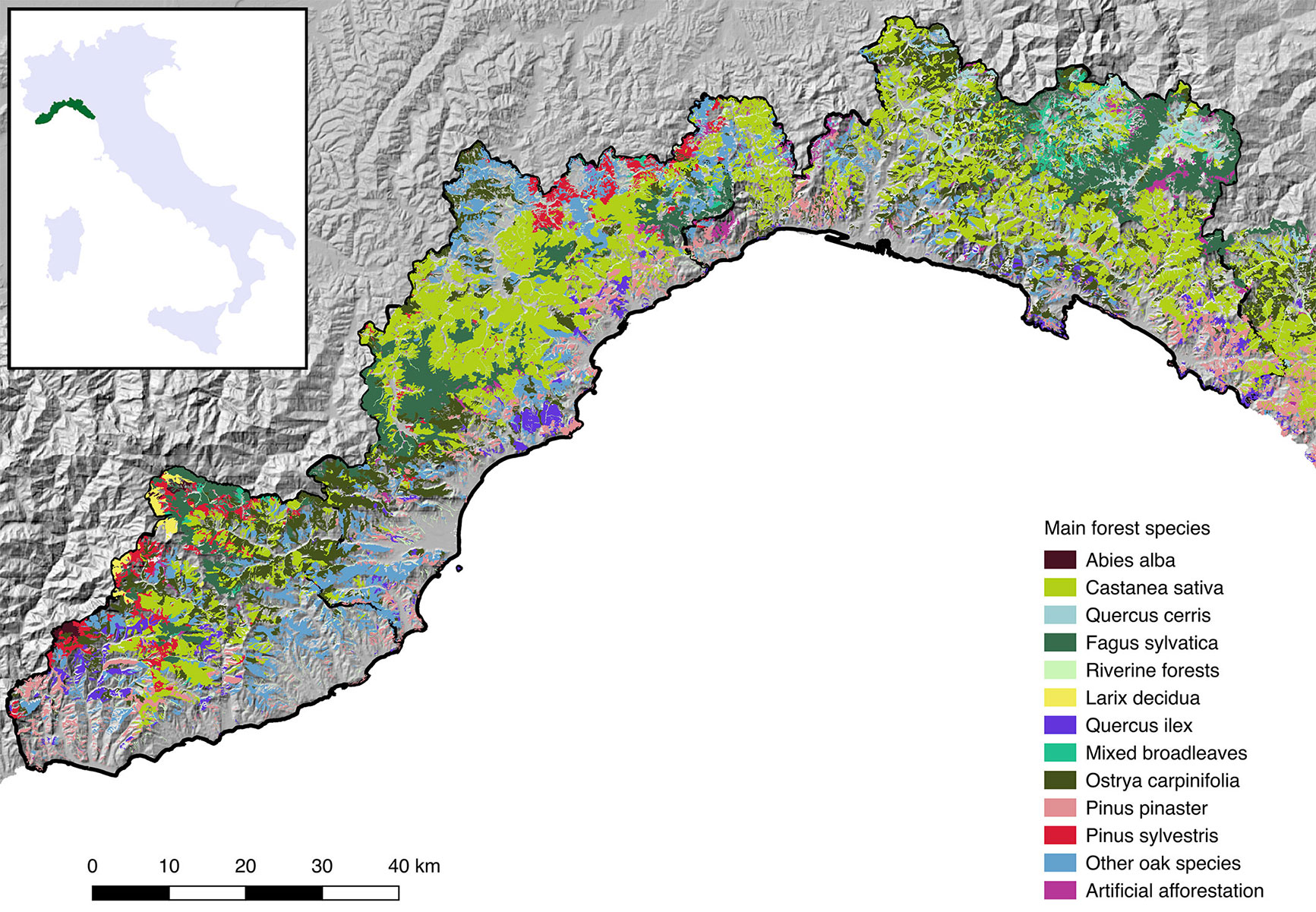
Image and data analysis
We chose one high-quality image (cloud cover <5%) acquired from Landsat 5 Thematic Mapper TM (path 194, row 029) on 7 June 1993, i.e., at the peak of the growing season, and contemporary to the last forest survey in which field plots were measured for the calibration of biomass models (see below). The image had a ground resolution of 30 m and was orthorectified based on the Advanced Spaceborne Thermal Emission and Reflection Radiometer Digital Elevation Model (ASTER DEM) with the same spatial resolution. The six reflective spectral bands (1-5, 7) of Landsat TM were converted to top-of-atmosphere reflectance and corrected for atmospheric thickness, with the thermal infrared band (6) serving as additional input for cloud masking ([7]).
Ground-based volume was predicted from data measured by the most recent regional forest inventory, which was carried out in 1993. The sampling design was two-phased; grid size for second phase plots (total number of plots = 1035) was 1 × 1 km, with concentric circular plots 200, 400, and 600 m2 in area for trees with a diameter at breast height (DBH) larger than 7.5, 12.5, and 17.5 cm, respectively. Species, forest cover type, DBH, and stem height were measured for all live trees inside each plot; species-specific and total tree volume (stem, branches, and foliage) was predicted as a function of DBH using national allometric models ([48]).
The statistical analyses used to model the relationships among spectral data and forest attributes should accommodate for the possibility that these relationships may be non-linear and complex ([23]). In order to deal with non-linear phenomena, a large array of statistical tools has been developed. Parametric models perform well in biomass estimation, especially with one or few predictors ([28]). However, they assume that the data follow some well-defined statistical distribution. Non-parametric models, on the other hand, do not require knowledge of the statistical distribution function of the response variable. Among non-parametric methods, artificial neural networks (ANN) integrate a cascade of simple non-linear computations that, when aggregated, can implement robust and complex non-linear functions, while adapting to any representative training set ([20]). In this work, we chose to test the performance of ANN for predicting the volume (subsequently converted to biomass) of broadleaf-dominated forests in a Mediterranean region where this technique had never been tested before.
A multilayer ANN consists of several simple processors called neurons, or cells, which are highly interconnected and are arranged in several computational steps or “layers”. The input and output layers can be connected directly, or through one or more intermediate calculation steps (“hidden layers” - [24]). The system works by predicting output data from patterns learned from a set of input training data. The difference between the current output layer and the fitted response is then used to adjust parameters (weights) within the network. The goal is to achieve a set of weights that reduces the error between observations and model output to less than a predetermined threshold ([24]). Once constructed, the ANN can be used to estimate or predict values for similar but unexperienced instances of the data.
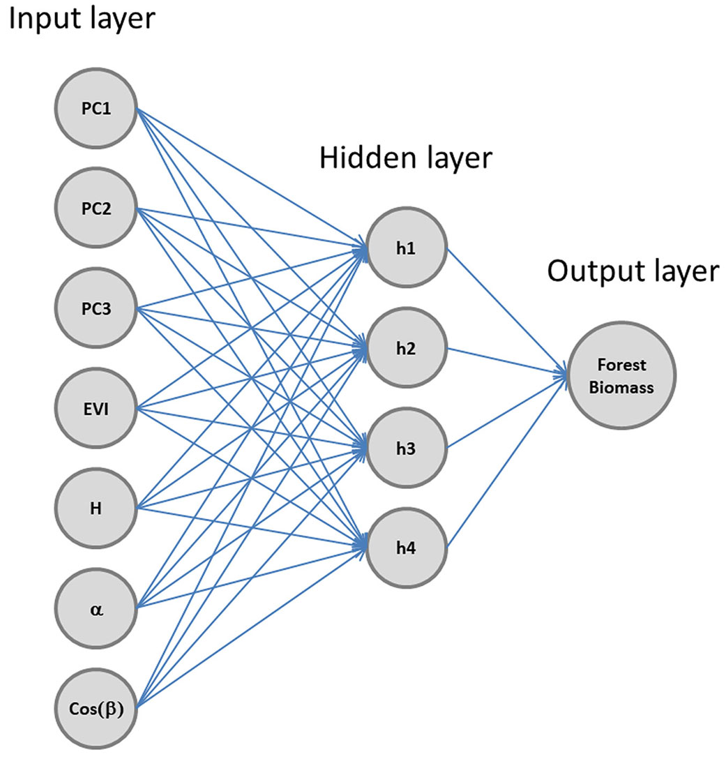
The main input to the ANN were the six reflective Landsat-TM bands. However, since Pearson’s correlation between any pair of bands across the image tile ranged from 0.50 to 0.98, a principal component transformation was applied. Additional input layers were elevation, slope, cosine of aspect generated from a 100 m Digital Elevation Model, and the Enhanced Vegetation Index ([22]) computed from Landsat-TM bands red, near infra-red, and blue. Relative to the commonly used Normalized Difference Vegetation Index (NDVI), EVI is characterized by a reduced influence of atmospheric conditions and canopy background signals and is more sensitive to leaf area index, stand and canopy structure ([22]). Small-volume plots (<50 m3 ha-1) were excluded from the training dataset. We used a multilayer Perceptron ANN ([17]) trained with a Levenberg-Marquardt Error Backpropagation (EBP) algorithm ([18]), and fitted the ANN separately for plots belonging to broadleaves- or conifers-dominated forest cover types (no mixed forest cover types existed in the regional classification - [6]). For each of the two groups, we divided field plots into a training (80%) and a validation (20%) set. The ANN had a single hidden layer of neurons (Fig. 2). The hyperbolic tangent and a linear function were selected as transfer functions in the hidden and the output layer, respectively. The Levemberg-Marquardt parameter was set to 0.001. A routine was in charge of repeating the training of the ANN and recording (in a report file) its performance when varying the numbers of hidden neurons from two to 15. The root mean square error (RMSE) was selected as the ANN performance parameter; it was estimated for both the training and the validation set ([27]). Volume per hectare was finally predicted for all 30-m pixels falling within polygons classified as conifers- or broadleaves-dominated forest cover types by the most recent regional forest inventory map ([6]). This map covered a total forested area of 223.985 ha, excluding woodlands and scrub (<10% forest cover by trees with height >3 m), and was created from visual photointerpretation of Quickbird® satellite imagery (pansharpened, false color composition from bands 4.3.2) using automatic object-oriented segmentation, classification based on 1217 field sampling plots where forest cover type was assigned depending on the species responsible for >50% canopy cover, and subsequent refinement with the aid of auxiliary information (i.e., maps from management plans, phenological information from multi-temporal pansharpened Landsat ETM7 imagery, lithologic maps). The complete methodology is described in Bocci & Vissani ([6]); the geometric precision of the map was 5m and the minimum mapping unit was 1.5 ha (but no validation statistics were reported by the source).
Fig. 2 - Multilayer Perceptron ANN with a single hidden layer, with input and output variables used in this study.
Available biomass supply
To demonstrate the practical relevance of wall-to-wall biomass mapping, we used the predicted volume to estimate the current supply of biomass residues available for bioenergy (i.e., tops and branches) across the study region. This required the following steps:
- update biomass estimates to the year when the bioenergy assessment is carried out, taking into account forest growth and losses due to natural or anthropogenic disturbances that have occurred in the meantime;
- select forests available for wood supply (FAWS - [1]);
- plan future harvest of wood for material purposes;
- estimate the biomass of harvest residuals produced according to the planned harvest scenarios.
In this demonstration, we assume that the bioenergy assessment must be carried out in the year 2005. This allowed to further improve the accuracy of our estimates by rescaling the updated pixel-level volume predictions obtained in (1) so as to be consistent with region-wide statistics of forest volume by cover type provided by the Italian National Forest Inventory for the same year. It was not possible to obtain volume estimates contemporary to the year of bioenergy assessment by using field-measured and remotely sensed data from 2005. In fact, although plot data from the Italian National Forest Inventory have recently been made available, the geographic precision of plot coordinates has been downgraded to 1 km, i.e., more than three orders of magnitude coarser than a Landsat pixel footprint, which we deem inadequate to accurately calibrate spatially-explicit volume prediction models.
For each pixel, forest volume was updated to the year 2005 by adding the current increment recorded for each forest cover type by the Italian National Forest Inventory for Liguria region ([16] - Tab. 1), times the number of years needed by the update (12). To account for the loss of standing volume due to harvest during the update period, we reduced current increment by 6.36% each year, following data on the average harvest intensity for the last decade in the region ([39]). Losses due to wildfire were estimated using regional data on mean yearly percent burned area by forest cover type ([39]); total burned area over the update period was converted into the loss of growing stock by assuming 100% mortality. Finally, we predicted loss due to pest and diseases by estimating the proportion of forest area described by the Italian National Forest Inventory as being damaged by “parasites” in the region and converted this into volume loss by assuming a mortality of 10%. Finally, to reconcile the updated pixel-level predictions with national forest inventory statistics, for each cover type we calculated the ratio of the average stock per hectare (sum of pixel volume divided by cover type area) to the average stock per hectare reported by the 2005 inventory (Tab. 1), and divided the volume in each pixel by such ratio, so that the sum of pixel volumes was equal to forest inventory estimates for each cover type.
Tab. 1 - Forest inventory data for the 13 main forest cover types in the study area, comparison between modeled and observed volume in 2005, and species-specific silvicultural and allometric parameters used in the analysis. (NFI): Italian National Forest Inventory; (A1993): area in 1993; (PV1993): predicted volume in 1993; (MPV1993): predicted volume per hectare in 1993; (CI2005): current increment from NFI in 2005; (BAY): area burned per year; (DA2005): area disturbed by pests and diseases in NFI 2005; (CIHY): current increment harvested per year; (PV2005): predicted volume per hectare updated for 2005; (MVNFI2005): volume per hectare from NFI in 2005; (PAV ratio 2005): predicted to actual volume ratio in 2005; (HI): harvest intensity; (RF) residue fraction; (BEF): biomass expansion factor; (WD): wood density.
| Main tree species |
Code | A1993 (ha) |
PV1993 (m3) |
MPV1993 (m3 ha-1) |
CI2005 (m3 ha-1 year-1) |
BAY(%) | DA2005 (%) |
CIHY (%) |
PV2005 (m3 ha-1) |
MVNFI2005 (m3 ha-1) |
PAV ratio 2005 |
HI | RF | BEF | WD (g cm-3) |
|---|---|---|---|---|---|---|---|---|---|---|---|---|---|---|---|
| Larix decidua | LC | 1.756 | 285.366 | 162.5 | 2.6 | 0.29 | 0.0 | 6.36 | 183.2 | 140.9 | 1.30 | 0.30 | 0.70 | 1.22 | 0.56 |
| Abies alba | AB | 680 | 152.535 | 224.3 | 11.7 | 0.29 | 0.0 | 6.36 | 333.8 | 398.5 | 0.84 | 0.30 | 0.84 | 1.34 | 0.38 |
| Pinus sylvestris | PM | 10.141 | 1.980.334 | 195.3 | 3.1 | 0.49 | 3.6 | 6.36 | 212.5 | 143.0 | 1.49 | 0.30 | 0.84 | 1.33 | 0.47 |
| Artificial afforestation | RI | 3.674 | 659.294 | 179.7 | 6.2 | 0.49 | 0.0 | 6.36 | 230.2 | 269.0 | 0.86 | 0.30 | 0.89 | 1.33 | 0.47 |
| Pinus pinaster | PC | 9.413 | 2.117.429 | 224.9 | 3.5 | 0.65 | 46.8 | 6.36 | 205.7 | 158.9 | 1.29 | 0.30 | 0.84 | 1.53 | 0.53 |
| Fagus sylvatica | FA | 27.457 | 6.829.051 | 248.7 | 5.4 | 0.31 | 1.0 | 6.36 | 293.0 | 216.4 | 1.35 | 0.35 | 0.25 | 1.36 | 0.61 |
| Other oaks | QU | 37.968 | 7.484.981 | 197.1 | 2.6 | 0.39 | 3.4 | 6.36 | 212.0 | 93.0 | 2.28 | 0.70 | 0.25 | 1.42 | 0.67 |
| Quercus cerris | CE | 328 | 73.019 | 222.6 | 3.9 | 0.39 | 0.0 | 6.36 | 251.5 | 159.6 | 1.58 | 0.70 | 0.25 | 1.45 | 0.69 |
| Castanea sativa | CA | 81.067 | 18.091.773 | 223.2 | 6.4 | 0.38 | 65.4 | 6.36 | 220.3 | 173.6 | 1.27 | 0.70 | 0.85 | 1.33 | 0.49 |
| Ostrya carpinifolia | OS | 41.387 | 8.565.890 | 206.8 | 3.3 | 0.35 | 0.8 | 6.36 | 231.1 | 89.7 | 2.58 | 0.70 | 0.25 | 1.28 | 0.66 |
| Riverine forests | FR | 3.787 | 781.064 | 206.3 | 5.0 | 0.35 | 0.0 | 6.36 | 247.8 | 165.9 | 1.49 | 0.70 | 0.25 | 1.39 | 0.41 |
| Mixed broadleaves | LM | 217 | 52.530 | 242.5 | 4.2 | 0.35 | 4.0 | 6.36 | 271.3 | 84.1 | 3.23 | 0.70 | 0.25 | 1.47 | 0.53 |
| Quercus ilex | LE | 6.110 | 1.041.243 | 170.4 | 2.7 | 0.45 | 2.6 | 6.36 | 186.9 | 80.7 | 2.32 | 0.70 | 0.25 | 1.45 | 0.72 |
Then, we selected FAWS by excluding pixels subject to special protection regimes (reserves, riparian areas up to 100 m from each stream or river), or inaccessible to logging equipment. Logging accessibility was excluded for slopes > 50% and for distances > 2500 m for any public road ([3]). Within such bounds, harvest was reduced using two coefficients equal to slope and distance from roads of each pixel relative to their maximum values ([3]). Vector layers for protected areas, rivers, and public roads were downloaded from an online regional cartographic database (⇒ http://www.cartografia.regione.liguria.it/).
To schedule silvicultural interventions for the next future (i.e., a 20-year period), local silviculturists were consulted to design the following sustainable management scheduled based on current forest structure, legal constraints (i.e., requirement to retain 60-80 standards ha-1 in coppices, 60-120 m3 ha-1 in even-aged forests, and 75-150 in uneven-aged forests -[43]), market demand, and criteria of ecological and economic sustainability: (i) conifer forests: group selection, 30% volume removed; (ii) beech coppices: conversion to high forest, 40% volume removed; (iii) beech high forests: selective thinning, 30% volume removed; (iv) other broadleaves: coppice with standards, 70% volume removed; (v) any pixel with volume < 100 m3 ha-1: no management in the next 20 years; (vi) any pixel belonging to Natura 2000 protected areas or in forests designated for direct protection from hydrogeological hazards: volume removed was further reduced by 25%.
Volume removed in the next 20 years was estimated based on the planned harvests and used to calculate available biomass of residues for energy use, by applying species-specific residue fractions drawn from available literature sources ([9], [30]) and corroborated by the opinion of local silviculturists regarding available harvest technologies and wood demand (hence the large fraction of conifer wood used for biomass - Tab. 1). Volume available for residues was finally converted to biomass by applying species-specific biomass expansion factors and wood density coefficients ([54] - Tab. 1).
Results
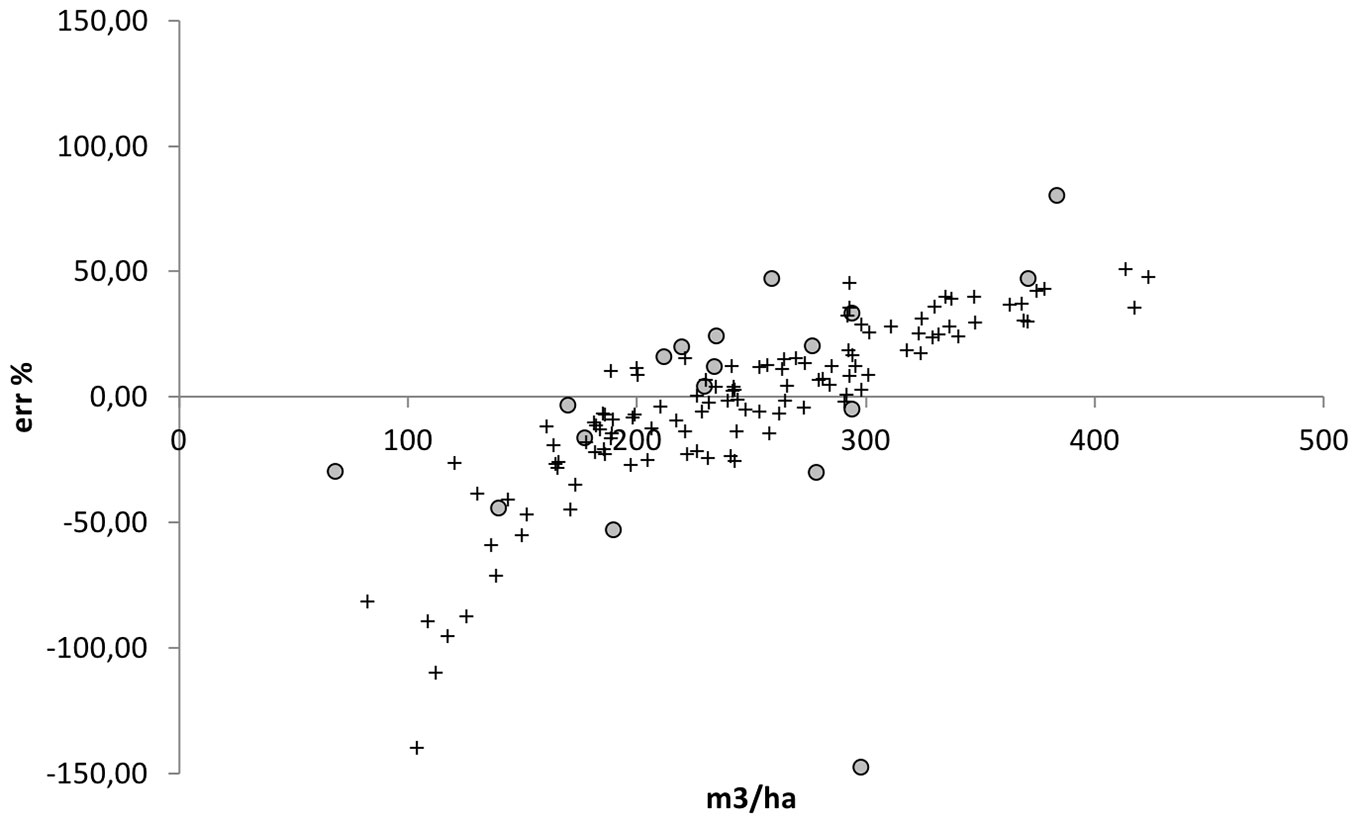
The six Landsat reflective bands were completely summarized by their first three principal components (cumulative variance explained = 99.95%). The first component was dominated by SWIR (eigenvector: +0.94), while the second and third components by green and red (Tab. 2). ANNs were trained on 539 broadleaves and 60 conifers plots (validation sets: 120 and 20 plots, respectively) using PC1, PC2, PC3, EVI, elevation, slope, and cos(Aspect) as predictors. The optimal networks had five and four nodes for broadleaves and conifers, respectively. Elevation, EVI, PC1, and PC3 were the most important variables in the broadleaves model, while EVI and PC2 were the main predictors for conifers (Tab. 3). The predicted aboveground volume was on average (± standard deviation) 214.1 ± 52.04 and 210.8 ± 215.54 m3 ha-1, for broadleaves and conifers respectively, with a mean percent error of -22.92% and -9.01% on the training set, and -23.86% and -27.18% on the validation set, for broadleaves and conifers respectively (Fig. 3). The standard deviation reported above was calculated from the distribution of ANN predictions over the entire study area and does not account for other sources of prediction uncertainty (see Discussions). Mean percent validation error was reduced to -2.2% and +9.7%, respectively when excluding very sparse or recently disturbed forests, i.e., those with standing volume <100 m3 ha-1 for broadleaves and <200 m3 ha-1 for conifers. The overall root mean square error for the calibrated estimate was 80.97 m3 ha-1; 95% confidence interval for the estimated mean volumes per hectare were 209.5 - 218.5 m3 ha-1 for broadleaves, and 154.8 - 267.2 m3 ha-1 for conifers.
Tab. 2 - Principal component analysis of Landsat 5 TM spectral bands.
| Band | Wavelength (mm) |
PC1 | PC2 | PC3 | PC4 | PC5 | PC6 |
|---|---|---|---|---|---|---|---|
| Blue | 0.42-0.52 | -0.0000 | -0.0042 | 0.0069 | -1.0000 | -0.0000 | -0.0000 |
| Green | 0.52-0.60 | 0.2435 | -0.6870 | 0.6846 | 0.0076 | 0.0000 | 0.0000 |
| Red | 0.63-0.69 | 0.2472 | -0.6386 | -0.7287 | -0.0024 | 0.0000 | -0.0000 |
| NIR | 0.76-0.90 | 0.0000 | -0.0000 | -0.0000 | -0.0000 | -0.3897 | 0.9210 |
| SWIR1 | 1.55-1.75 | 0.0000 | -0.0000 | -0.0000 | -0.0000 | 0.9210 | 0.3897 |
| SWIR2 | 2.08-2.35 | 0.9379 | 0.3467 | 0.0143 | -0.0014 | -0.0000 | 0.0000 |
| Variance (%) | - | 45.0 | 51.3 | 3.6 | 0.1 | 0.0 | 0.0 |
| Cum. variance (%) | - | 45.0 | 96.3 | 99.9 | 100.0 | 100.0 | 100.0 |
Tab. 3 - ANN statistics and weights for broadleaves and conifers.
| Group | Weights (w) | Node | PC1 | PC2 | PC3 | EVI | Elevation | Slope | cos(Aspect) |
|---|---|---|---|---|---|---|---|---|---|
| Broadleaves | Absolute input w | node 1 | 49.85 | 160.88 | -22.62 | 220.89 | 21.72 | 231.31 | -249.45 |
| node 2 | -6.02 | -0.43 | -6.26 | -6.45 | 7.95 | -5.27 | -1.21 | ||
| node 3 | -605.47 | 247.08 | 48.26 | -139.85 | 157.61 | 141.82 | -62.15 | ||
| node 4 | -0.24 | 60.21 | -44.45 | 59.92 | 24.4 | 21.77 | -5.41 | ||
| node 5 | 6.13 | 0.74 | 6.49 | 6.96 | -8.19 | 5.36 | 1.25 | ||
| Relative input w (%) | node 1 | 5.20 | 16.80 | 2.40 | 23.10 | 2.30 | 24.20 | 26.10 | |
| node 2 | 17.90 | 1.30 | 18.60 | 19.20 | 23.70 | 15.70 | 3.60 | ||
| node 3 | 43.20 | 17.60 | 3.40 | 10.00 | 11.20 | 10.10 | 4.40 | ||
| node 4 | 0.10 | 27.80 | 20.50 | 27.70 | 11.30 | 10.10 | 2.50 | ||
| node 5 | 17.50 | 2.10 | 18.50 | 19.80 | 23.30 | 15.30 | 3.60 | ||
| Total w | - | 17.62 | 1.95 | 18.43 | 19.54 | 23.27 | 15.48 | 3.72 | |
| Output | Output 1 | Output 2 | Output 3 | Output 4 | Output 5 | - | - | ||
| A bsolute output w | 0.19 | 15.4 | -0.1 | 0.14 | 15.1 | - | - | ||
| R elative output w (%) | 0.60 | 49.80 | 0.30 | 0.40 | 48.80 | - | - | ||
| Conifers | Absolute input w | node 1 | 46.43 | 170.93 | -26.41 | 142.87 | 4.26 | -28.08 | -21.43 |
| node 2 | -211.11 | 149.55 | 8.44 | 112.6 | 9.49 | 115.44 | -99.6 | ||
| node 3 | 45.83 | 166.19 | -25.07 | 140.46 | 3.94 | -25.96 | -20.54 | ||
| node 4 | -186.98 | 79.82 | 10.35 | 73.26 | 125.62 | -193.19 | -56.27 | ||
| Relative input w (%) | node 1 | 10.50 | 38.80 | 6.00 | 32.40 | 1.00 | 6.40 | 4.90 | |
| node 2 | 29.90 | 21.20 | 1.20 | 15.90 | 1.30 | 16.30 | 14.10 | ||
| node 3 | 10.70 | 38.80 | 5.90 | 32.80 | 0.90 | 6.10 | 4.80 | ||
| node 4 | 25.80 | 11.00 | 1.40 | 10.10 | 17.30 | 26.60 | 7.80 | ||
| Total w | - | 10.75 | 38.64 | 5.89 | 32.48 | 1.01 | 6.34 | 4.88 | |
| Output | Output 1 | Output 2 | Output 3 | Output 4 | - | - | - | ||
| A bsolute output w | 34.77 | 0.25 | -34.99 | -0.29 | - | - | - | ||
| R elative output w (%) | 49.50 | 0.30 | 49.80 | 0.40 | - | - | - | ||
Fig. 3 - Percent validation error for remote-sensing biomass assessment in broadleaves- (crosses) and conifers- (circles) dominated plots.
After predicting volume in year 1993 for all pixels of the study region, updating it based on forest growth and losses, and averaging it over all the area covered by each forest type, we obtained estimates of the growing stock that were overestimating NFI data by 56% (average weighted over the area covered by each forest cover type. Errors ranged from 16% underestimation in Abies alba to 223% overestimation in mixed broadleaves forests (Tab. 1). However, this forest cover types occupy a very small proportion of the landscape. Large prediction errors might be related to unforeseen forest disturbances that have occurred during the update period.
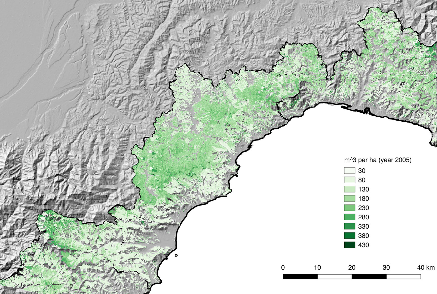
After normalizing on national forest inventory statistics, mean aboveground forest volume ranged from 81 to 391 m3 ha-1 (cell mean = 147.3 m3 ha-1, cell st.dev. = 84.6 m3 ha-1 - Fig. 4), and was generally large (but also more uncertain, as suggested by a much larger coefficient of variation) for conifers than for broadleaves (Tab. 4).
Fig. 4 - Modeled dendrometric volume (over bark) in the study area after ANN fitting, updating to 2005, and normalizing on species-specific NFI aggregate volume.
Tab. 4 - Forest available for wood supply, harvested volume, and biomass harvested for wood supply in a 20-year period for each forest cover type in the study area. (NMV): modeled volume, normalized; (HV): harvested volume; (HR): Harvest rate; (Tot. Biomass): total biomass for bioenergy; (Mean Biomass): mean biomass for bioenergy; (STD): standard deviation.
| Code | Area (ha) |
FAWS (ha) |
FAWS (%) |
NMV (m3 ha-1) |
HV (m3 ha-1) |
HR (%) |
Tot Biomass (Mg) |
Mean biomass (Mg ha-1) |
||||||
|---|---|---|---|---|---|---|---|---|---|---|---|---|---|---|
| Mean | STD | Mean | STD | Mean | STD | Max | Mean | STD | Max | |||||
| LC | 1.756 | 1.011 | 58 | 151.9 | 194.2 | 8.6 | 14.6 | 5.5 | 3.9 | 27.7 | 2.668.4 | 2.6 | 5.7 | 69.3 |
| AB | 680 | 0 | 0 | 398.4 | 157.4 | 0 | 0 | 0.0 | 0.0 | 0.0 | 0.0 | 0.0 | 0.0 | 0.0 |
| PM | 10.141 | 6.695 | 66 | 145.8 | 134.3 | 14.7 | 20.5 | 9.8 | 7.1 | 68.5 | 40.140.3 | 6 | 9.4 | 254.6 |
| RI | 3.674 | 2.144 | 58 | 280.7 | 222.5 | 24.7 | 30.2 | 9.1 | 6.9 | 66.6 | 24.307 | 11.3 | 11.8 | 168.9 |
| PC | 9.413 | 5.052 | 54 | 155.5 | 150.7 | 16.4 | 22.3 | 10.8 | 6.9 | 68.5 | 39.116.4 | 7.7 | 11.7 | 198.5 |
| QU | 27.457 | 24.361 | 89 | 93.2 | 22.6 | 20.8 | 14.9 | 22.3 | 14.6 | 69.7 | 64.816.1 | 2.7 | 4.1 | 164.3 |
| FA | 37.968 | 18.209 | 48 | 216.7 | 44.5 | 15.7 | 13 | 7.3 | 5.9 | 65.1 | 62.550.8 | 3.4 | 3.4 | 67.4 |
| CE | 328 | 175 | 53 | 158.8 | 37.6 | 26.7 | 21.5 | 16.9 | 13.3 | 64.3 | 1.150.7 | 6.6 | 9.1 | 62.6 |
| CA | 81.067 | 53.627 | 66 | 173.8 | 35.2 | 37.1 | 25.6 | 21.3 | 14.1 | 69.2 | 993.041.7 | 18.5 | 13.4 | 150.7 |
| OS | 41.387 | 23.787 | 57 | 89.9 | 21 | 17.3 | 13.3 | 19.3 | 14.1 | 68.9 | 44.473.4 | 1.9 | 3.6 | 90.3 |
| FR | 3.787 | 1.659 | 44 | 169.8 | 76.8 | 37.2 | 31.8 | 21.5 | 14.7 | 66.9 | 14.470.3 | 8.7 | 10.4 | 129.3 |
| LM | 217 | 132 | 61 | 84.6 | 33.1 | 11 | 13.5 | 13.3 | 13.0 | 61.8 | 597.3 | 4.5 | 7.6 | 55.8 |
| LE | 6.110 | 3.043 | 50 | 80.8 | 21.2 | 18.5 | 12.9 | 22.8 | 14.2 | 68.3 | 3.955.2 | 1.3 | 3.1 | 88.2 |
| Total | 200.007 | 139.894 | 70 | 146.6 | 84.6 | 25.2 | - | 18.1 | - | 70.0 | 1.295.921.6 | 9 | - | 254.6 |
FAWS (slope <50%, distance from any public road <2500 m, distance from rivers >100 m) covered 140,357 ha (70% of forested area). Planned volume removals per pixel ranged from 0 to 947.8 m3 ha-1 (mean: 25.4 m3 ha-1, or 18.7% of the average standing stock across FAWS); pixel-level estimates are bound to be affected by large uncertainties, but silvicultural planning is usually carried out at the level of management unit that are several hectares in size and include hundreds of Landsat pixels, so that locally large errors will be diluted.
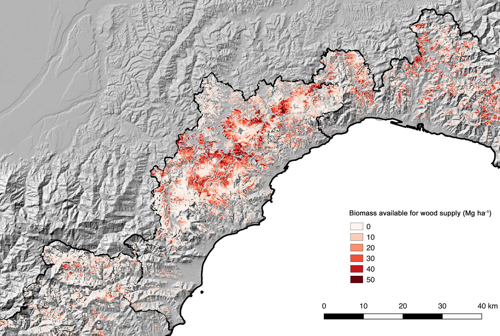
After applying species-specific residue fractions and converting to dry matter units, biomass available for bioenergy supply was estimated to be 1,295,921 million Mg dry matter, or 8.95 Mg ha-1 (Fig. 5).
Fig. 5 - Removed biomass (dry matter units) predicted for FAWS in the study area.
Discussion
The modeling part of the study used state-of-the-art algorithm to calibrate and correct remotely sensed images. By fitting separate models on conifers and broadleaves, and using a non-parametric, adaptive learning algorithm, capable of handling non-linearity and threshold relationships, we were able to estimate forest volume with a mean validation error of -23% and -27% respectively across a large region (before updating). While in local studies the relationships between remotely sensed imagery and volume or biomass may attain a goodness-of-fit larger than 0.70, and up to 0.98 ([14]), such accuracy in a variable that is not directly “seen” from satellite sensors is uncommon for estimates of volume spanning large areas and forests with different species composition ([55]) and management type (high forests and coppices). Data fusion between model-assisted estimates and national forest inventory statistics at the provincial level helped increase the accuracy of volume estimates and made them consistent with official forest statistics.
Principal component analysis of Landsat bands helped avoided collinearity in the model structure. Elevation, slope, EVI, and PC1 were the most important predictors in the volume modeling algorithm. The importance of elevation (especially in broadleaves) and of slope conforms to an expected topographical gradient of site productivity (smallest on steeper slopes). EVI is directly linked to photosynthetic activity and leaf area and is immune from saturation problems that affect the more commonly used NDVI ([22]). Finally, PC1 is dominated by the SWIR2 band (Tab. 1), which was highlighted by several recent studies as a robust predictor of aboveground biomass and forest structure, with a negative correlation to such variables ([56]).
In the study area, the volume of conifers was estimated more accurately but at the same time it exhibited more variability from pixel to pixel than broadleaves (coefficient of variation: 102%). This is likely a reflection of the large topographic and vegetational diversity of the study area, where conifer forests include both sparse stands of shade-intolerant Mediterranean pine stands, where standing volume can be heavily impacted by fire or pest and diseases ([32]), as well as high-elevation mountain conifer forests dominated by European larch (Larix decidua Mill.) and artificially established Norway spruce (Picea abies Karst) that, if left unmanaged for several decades, exhibit very large standing stocks. Since in such cases the most viable management option is selection thinning, most of the standing stock in these untended, low-quality timber stands is likely going to be used as energy wood. By comparison, the growing stock of broadleaves forests is smaller, as a result of the prevalence of coppiced or formerly coppiced stands - with the exception of beech, which has in most cases overcome the maximum age allowed for coppicing (40 years - [51]) and is mostly managed as high forests.
In the second part of this study, we used the predicted volume to obtain estimates of aboveground biomass, which we then coupled with site and technical availability of forests for wood supply, and with a realistic, sustainable, and locally determined silvicultural schedule for the next 20 years, to obtain an estimate of biomass actually available for energy supply. The workflow used to update volume and estimate harvestable biomass from FAWS may help tactical planning of biomass supply and energy/heating plant establishment. Such approach is reproducible wherever aggregated inventory data and geographical layers are available. Planned harvest intensities took into account current forest practice, historical harvest rates, as well as legal limitations and best practices to ensure the simultaneous provision of wood and other ecosystem services, e.g., carbon stocking ([52]) or hydrogeologic protection ([50]).
We estimated how much biomass would be harvestable in the next two decades by using a “stock change” approach, e.g., planning one-off silvicultural entries and estimating the removed volume, rather than assessing removals based on estimated future woody increment ([47]). Our approach is applicable in all cases where not all forests are managed, and where no harvest planning exists at the regional level, something that precludes any assumption on a predetermined balance between increment and removals. If prediction needs to be carried out on longer time scales, such approach should be replaced by more comprehensive modeling tools ([53]) which are capable of tracking the complex age-structure feedbacks that affect forests undergoing management for more than one rotation.
The assessment carried out in this study is affected by several uncertainties. From the point of view of prediction accuracy (i.e., the degree to which the predictions reflect reality), the mean relative error of the predictions of the volume model was between -20 and -30% of plot-based forest volume across the whole validation dataset, and only -2 to +10% when excluding very sparse or young forests, which should not undermine the accuracy of the predicted biomass map for the intended purpose. On the other hand, the precision of volume predictions (i.e., the uncertainty associated with the width of confidence intervals) was in some case quite low, for example in the case of broadleaves where the standard deviation of volume predictions was higher than their mean. However, this can be due to the wide variety of forest types and structures included in the “broadleaves” class, which range from dense, overmature beech coppices to sparse oak forests. Finally, the estimation of current biomass required additional steps, assumptions, and data fusion, such as allometric model predictions, use of auxiliary data to refine forest cover typing, updating estimates to the assessment year, estimating harvest reductions, excluding sparse forests. All of these sources contributed to greater uncertainty in both the map and the estimates obtained from the map, although often by an undefined amount.
In particular, the rescaling of pixel-level volumes, based on the total volumes reported for each forest cover type in the study region, made sure that the aggregated error at forest type level was zero, at least in areas not damaged by natural disturbances (insects, wildfire) in the period 1993-2005. As pixel-level estimates likely remained affected by an error of a magnitude similar to that before updating (RMSE: 90 m3 ha-1), an ad-hoc validation sampling should be carried out by establishing new forest plots where biomass is evaluated in the supply area before designing detail supply plans for any individual biomass plant.
Once equipped with a high-resolution, wall-to-wall estimate of forest biomass available for energy (Fig. 5), stakeholders and investors can use these data to decide upon the location and power of biomass energy plants. We estimated 1.300.000 Mg of fresh biomass available in the next 20 years, corresponding to nearly 250,000 TOE or 12,500 TOE year-1. Using the assumptions presented in the regional Energy and Environmental Plan ([44]), this corresponds to an installed power of 121 MW, or about 24 new biomass energy plants with a power of 5 MW. Our analysis showed that, when taking into account only biomass from forestry residues, and fully considering limitations to biomass supply due to the accessibility of protected area status, the goal of a three-fold increase in power installed in biomass plants is not attainable using sustainably harvested local resources.
To decide on the localization of such plants, however, assessing biomass availability is a prerequisite, but additional factors tied to demand side will need to be taken into consideration which were not included in this study, such as annual woodchips consumption per plant type (heating, CHP, electricity), range of short supply lines, spatial and temporal characteristics of energy demand (both thermal and electrical), infrastructures for district heating and logistics for biomass processing pre-treatment, space availability for biomass storage and conversion, and additional energy sources available to each municipality or district. Tools have been developed that take such factors into considerations, such as Biomassfor ([47]) and the BeWhere model ([25]). The latter, in particular, identifies the optimal geographical locations, capacities, technologies, and a number of bioenergy production plants, while keeping track of the costs, emissions, and energy quantities of each segment of the supply chain. Therefore, for each scenario produced, the renewable energy potential, the power production cost, and the avoided emissions can be forecasted.
References
CrossRef | Gscholar
CrossRef | Gscholar
CrossRef | Gscholar
Online | Gscholar
CrossRef | Gscholar
CrossRef | Gscholar
CrossRef | Gscholar
Gscholar
Gscholar
Online | Gscholar
CrossRef | Gscholar
Gscholar
Gscholar
Gscholar
CrossRef | Gscholar
Gscholar
Gscholar
Authors’ Info
Authors’ Affiliation
Università degli Studi di Milano, DISAA, v. Celoria 2, I-20123 Milano (Italy)
Renzo Motta
Enrico Mondino Borgogno
Università degli Studi di Torino, DISAFA, l.go Braccini 2, I-10095 Grugliasco, TO (Italy)
Corresponding author
Paper Info
Citation
Vacchiano G, Berretti R, Motta R, Mondino Borgogno E (2018). Assessing the availability of forest biomass for bioenergy by publicly available satellite imagery. iForest 11: 459-468. - doi: 10.3832/ifor2655-011
Academic Editor
Rodolfo Picchio
Paper history
Received: Oct 18, 2017
Accepted: Apr 17, 2018
First online: Jul 02, 2018
Publication Date: Aug 31, 2018
Publication Time: 2.53 months
Copyright Information
© SISEF - The Italian Society of Silviculture and Forest Ecology 2018
Open Access
This article is distributed under the terms of the Creative Commons Attribution-Non Commercial 4.0 International (https://creativecommons.org/licenses/by-nc/4.0/), which permits unrestricted use, distribution, and reproduction in any medium, provided you give appropriate credit to the original author(s) and the source, provide a link to the Creative Commons license, and indicate if changes were made.

Web Metrics
Breakdown by View Type
Article Usage
Total Article Views: 38802
(from publication date up to now)
Breakdown by View Type
HTML Page Views: 33662
Abstract Page Views: 1916
PDF Downloads: 2566
Citation/Reference Downloads: 7
XML Downloads: 651
Web Metrics
Days since publication: 2124
Overall contacts: 38802
Avg. contacts per week: 127.88
Article Citations
Article citations are based on data periodically collected from the Clarivate Web of Science web site
(last update: Feb 2023)
Total number of cites (since 2018): 5
Average cites per year: 0.83
Publication Metrics
by Dimensions ©
Articles citing this article
List of the papers citing this article based on CrossRef Cited-by.
Related Contents
iForest Similar Articles
Research Articles
A geographically weighted deep neural network model for research on the spatial distribution of the down dead wood volume in Liangshui National Nature Reserve (China)
vol. 14, pp. 353-361 (online: 27 July 2021)
Review Papers
Remote sensing-supported vegetation parameters for regional climate models: a brief review
vol. 3, pp. 98-101 (online: 15 July 2010)
Research Articles
Identification of wood from the Amazon by characteristics of Haralick and Neural Network: image segmentation and polishing of the surface
vol. 15, pp. 234-239 (online: 14 July 2022)
Research Articles
Estimation of aboveground forest biomass in Galicia (NW Spain) by the combined use of LiDAR, LANDSAT ETM+ and National Forest Inventory data
vol. 10, pp. 590-596 (online: 15 May 2017)
Research Articles
Artificial intelligence associated with satellite data in predicting energy potential in the Brazilian savanna woodland area
vol. 13, pp. 48-55 (online: 05 February 2020)
Research Articles
Afforestation monitoring through automatic analysis of 36-years Landsat Best Available Composites
vol. 15, pp. 220-228 (online: 12 July 2022)
Research Articles
Modelling dasometric attributes of mixed and uneven-aged forests using Landsat-8 OLI spectral data in the Sierra Madre Occidental, Mexico
vol. 10, pp. 288-295 (online: 11 February 2017)
Review Papers
Accuracy of determining specific parameters of the urban forest using remote sensing
vol. 12, pp. 498-510 (online: 02 December 2019)
Review Papers
Remote sensing of selective logging in tropical forests: current state and future directions
vol. 13, pp. 286-300 (online: 10 July 2020)
Research Articles
Assessing water quality by remote sensing in small lakes: the case study of Monticchio lakes in southern Italy
vol. 2, pp. 154-161 (online: 30 July 2009)
iForest Database Search
Search By Author
Search By Keyword
Google Scholar Search
Citing Articles
Search By Author
Search By Keywords
PubMed Search
Search By Author
Search By Keyword


