Sensitivity analysis of RapidEye spectral bands and derived vegetation indices for insect defoliation detection in pure Scots pine stands
iForest - Biogeosciences and Forestry, Volume 10, Issue 4, Pages 659-668 (2017)
doi: https://doi.org/10.3832/ifor1727-010
Published: Jul 11, 2017 - Copyright © 2017 SISEF
Research Articles
Abstract
This study investigated the statistical relationship between defoliation in pine forests infested by nun moths (Lymantria monacha) and the spectral bands of the RapidEye sensor, including the derived normalized difference vegetation index (NDVI) and the normalized difference red-edge index (NDRE). The strength of the relationship between the spectral variables and the ground reference samples of percent remaining foliage (PRF) was assessed over three test years by the Spearman’s ρ correlation coefficient, revealing the following ranking order (from high to low ρ): NDRE, NDVI, red, NIR, green, blue, and red-edge. A special focus was directed at the vegetation indices. In both discriminant analyses and decision tree classification, the NDRE yielded higher classification accuracy in the defoliation classes containing none to moderate levels of defoliation, whereas the NDVI yielded higher classification accuracy in the defoliation classes representing severe or complete defoliation. We concluded that the NDRE and the NDVI respond very similarly to changes in the amount of foliage, but exhibit particular strengths at different defoliation levels. Combining the NDRE and the NDVI in one discriminant function, the average gain of overall accuracy amounted to 7.8 percentage points compared to the NDRE only, and 7.4 percentage points compared to the NDVI only. Using both vegetation indices in a machine-learning-based decision tree classifier, the overall accuracy further improved and reached 81% for the test year 2012, 71% for 2013, and 79% for the test year 2014.
Keywords
Forest Health, Discriminant Analysis, Pine Defoliation, Normalized Difference Red-edge Index, Decision Tree Classification
Introduction
Insect defoliation is a frequent and recognized problem in the world’s managed forests, particularly in industrial plantations and homogeneously structured forests. The FAO’s Global Forest Resources Assessment 2010 ([18]) reports the ten most prevalent insect pests in Europe of which two are bark beetle species and eight are defoliators. According to the FAO’s Global Forest Resource Assessment main report ([16]), 1.870.000 km² of the world’s forests are plantations, which represent about 5% of the estimated global total forest area. The principle genera grown in plantations worldwide are Pinus (20%) and Eucalyptus (10%). In Germany, Scots pine (Pinus sylvestris) occupies 24% of the total forest area ([19]). Conifer plantations commonly consist of one species and are therefore particularly prone to mass outbreaks of pests like defoliating insects, since uniform structure and species poorness do not provide as much ecological niches for natural antagonists as mixed and structure rich forests ([33]). The greater the number of plant and animal species that inhabit an ecosystem, the greater are the barriers and balances that prevent any one species from increasing to the point where other ecosystem components are threatened ([17]). Economic damages result from necessary additional investments in phytosanitary measures - for instance, insecticide applications or removal of dead trees. If trees survive, slowed growth of wood from reduced photosynthesis activity induces indirect economic damage. Thus, the monitoring of affected forest areas and the mapping and estimation of the defoliation extent and magnitude is important for both forest managers and forest ecologists ([39]). In Germany, five pest species (orders Lepidoptera and Hymenoptera) are common in Scots pine plantations. They are often referred to as grand pine defoliators because of their repetitive mass outbreaks ([33])
Several studies considering a variety of sensors and methods have suggested the capabilities of optical satellite remote sensing for defoliation mapping ([39], [24], [46], [12], [9], [50], [1], [44]). To understand how satellite remote sensing can be used to detect or assess defoliation, it is important to review the interaction of light and vegetation in general, and the forest canopy in specific. Leaves of healthy vegetation absorb light for photosynthesis in the visible region of the electromagnetic spectrum, particularly in the blue, red-orange, red, and a smaller amount in the red-edge wavelengths. Absorption in the green part of the spectrum takes place but is rather weak ([38]). The NIR band interacts with healthy leaf structure and is scattered by the air-cell interfaces of the spongy mesophyll ([29]). Sensitivity of the red-edge portion of the electromagnetic spectrum to variations in leaf chlorophyll content was reported first by Rabinowitch & Govindjee ([38]) who pointed out the existence of a chlorophyll absorption peak at 695 nm. Evidence for this hypothesis was for instance provided by Gitelson et al. ([20]). As the needle mass is reduced, chlorophyll absorption decreases, causing an increase of reflectance in the chlorophyll absorption bands. Simultaneously, biomass of healthy leaves is reduced leading to a decrease in the NIR reflectance.
Leaf Area Index (LAI) is strongly related to the varying amount of foliage in the canopy ([42]). Barclay & Goodman ([3]) and Zeng & Moskal ([57]) report five different measures of LAI. Chen & Black ([10]) specified the LAI for conifers (non-flat leaves) as half the total intercepting area per unit ground surface area. If it is the aim to estimate the LAI using optical satellite imagery, ground reference data needs to be collected and related to spectral variables (spectral bands or vegetation indices) in order to build, for example, linear or non-linear regression models ([43], [45], [48]). The collection of LAI samples can occur directly (e.g., leaf collection) or with indirect non-contact methods which rely on suitable devices like the Licor LAI-2000 Plant Canopy Analyzer or optical camera systems for hemispherical photography. Detailed information about devices and methods can be found in Jonckheere et al. ([30]) and Homolová et al. ([26]). Therefore, LAI sampling must be considered a fairly time consuming and costly procedure. Bréda ([6]) pointed out that remotely sensed vegetation indices at present would need a site- and stand-specific calibration against ground-based measurements of LAI and still do not yield suitable results for complex canopies such as forests. Therefore, it would be necessary to rely first on qualitatively sufficient ground-based LAI estimates.
In contrast, visual estimation of percent remaining foliage (PRF) is rather inexpensive and can efficiently be implemented. In fact, visual assessment of tree defoliation is often applied in the practice for forest health assessment in Germany, unlike LAI. In the ICP Forest (International Co-operative Programme on Assessment and Monitoring of Air Pollution Effects on Forests) crown condition assessment, defoliation taxation is implemented by using foliage transparency as a proxy variable which is visually estimated in 5% intervals ([27]). This approach was developed by Tallent-Halsell ([49]).
The number of studies relating optical satellite remote sensing and insect defoliation is comparably low and often based on freely available imagery at medium to low spatial resolution. Hall et al. ([22]) evaluated the performance of the Landsat TM sensor in detecting tree top kill caused by the Jack pine budworm (Choristoneura pinus pinus) in a three-year time series. They found poor spectral differences in the bands of Thematic Mapper data related to defoliation intensities in the studied stands. Correlations between NDVI and defoliation were not as high as in other existing studies, and this was attributed to the interfering signals from the ground vegetation of the relatively open forest canopy. Falkenström & Ekstrand ([15]) correlated Norway spruce and Scots pine defoliation samples with the IRS-LISS III sensor spectral bands, band ratios and vegetation indices. They reported the highest correlations for the NIR band (r= -0.83), the NIR/red-ratio (r= -0.92), and the NDVI (r= -0.91) in almost pure pine stands. De Beurs & Townsend ([12]) tested MODIS-based composite NDVI, EVI (Enhanced Vegetation Index), Normalized Difference Water index (NDWI), and two other Short Wave Infrared band (SWIR) based indices (NDIIb6 and NDIIb7) for their capacity to map gypsy moth (Lymantria dispar) defoliation as estimated by ground observations. They concluded that defoliation estimates based on NDIIb6 and NDIIb7 can be reliably used to monitor insect defoliation annually at a minimum mapping unit of 0.63 km². Using Landsat TM data and applying spectral mixture analysis and determinant separation, Radeloff et al. ([39]) suggested the possibility of mapping defoliation by Jack pine budworm with high accuracies. Hall et al. ([23]) correlated ground-based with satellite-based (Landsat ETM+) relative LAI estimates to map defoliation in aspen (Populus ssp.) stands caused by the large aspen tortrix (Choristoneura conflictana). Their correlation analysis resulted in a Pearson’s correlation coefficient of 0.84. High and very high resolution imagery provide better spatial detail for defoliation mapping, however, there have not a lot of studies been published so far, probably because such data is usually not freely available. Adelabu et al. ([1]) compared Support Vector Machine and Random Forest classifiers for the segregation of three defoliation classes with 5 m multi-spectral RapidEye imagery in a study area situated in the Mopane woodland in Botswana. The presence of the RapidEye red-edge band led to an increase in classification accuracy of about 20 percent points using both of the above methods. Furthermore, they observed a better separation of the defoliation classes by the NDRE than by the NDVI. Chávez & Clevers ([9]) used multi-spectral WorldView2 data (2 m spatial resolution) to evaluate the health condition of savannah trees characterized by 5 classes of green canopy percentage (GC%). The comparison of the NDRE and the NDVI indicated significant correlations with GC% for both vegetation indices, with a higher Spearman’s ρ coefficient of 0.91 for the NDVI. The Spearman’s ρ for the NDRE was 0.83.
The purpose of this study was to analyze the statistical relationship between defoliation in Scots pine plantations and the five RapidEye bands, as well as the derived spectral indices NDVI and NDRE, by means of different methods of analytical statistics. Correlation and discriminant analysis (DA) were used to assess the statistical trends between the variables over three consecutive years (2012, 2013, and 2014). Eventually, a machine-learning based DTC (decision tree classifier) was applied and its classification outcome related to the previously observed results. A special focus was put on the comparison of the NDRE and the NDVI, since the NDVI is a traditionally and frequently used vegetation index, while the broad band NDRE is specific only for a few optical satellite systems, namely RapidEye, Sentinel 2A, WorldView-2, and WorldView-3. In this regard, a generic aim of the analysis was to positively contribute to the research presented in other existing studies investigating and comparing the NDVI and NDRE for vegetation monitoring, in particular forest health monitoring. Considering the depth of the analysis and pine plantation as the studied vegetation type, no such study specific for the RapidEye sensor can be found so far in the literature.
Materials and methods
Test sites
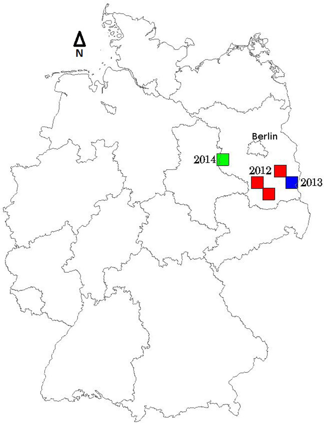
The test sites were situated in the southeast of the federal state Brandenburg, Germany (Fig. 1). The area is characterized by flat terrain with Scots pine forest plantations (Pinus sylvestris) growing mainly on poor sandy soils. The water holding capacity of the soils is low. Canopies of the pine forest are relatively homogeneous and therefore, spectrally almost uniform. However, some variation is still present due to differences in age, growth stages and canopy densities of different plantation compartments. Plant associations within the pine plantations include: Dryopteri-Cultopinetum sylvestris with dense fern ground vegetation, Calamagrostio-Cultopinetum sylvestris vegetated chiefly with reed grasses, Calluno-Cultopinetum sylvestris with a mixture of heather and mosses, and Molinio-Myrtillo-Cultopinetum sylvestris where blueberry shrubs grow together with wood sorrel and moor grasses ([25]). Inter-mixed tree species are sessile oak (Quercus petraea), birch (Betula pendula), and black locust (Robinia pseudoacacia). A nun moth (Lymantria monacha) outbreak occurred between 2011 and 2014 is currently in the retro-gradation phase. Symptoms for a commencing pine tree lappet moth (Dendrolimus pini) gradation were observed in 2014.
Fig. 1 - Location of RapidEye test tiles located in the federal state Brandenburg (52° 07′ 53.0″ N 13° 12′ 58.3″ E), Northeast Germany, map scale: 1:5.000.000.
RapidEye imagery
In this study, RapidEye data from 2012, 2013, and 2014 were used. Nun moth caterpillars cease feeding approximately in mid-July and emerge as adult butterflies after a few days of pupation ([33]). Hence, defoliation can be most reliably assessed only towards the end of July. Tab. 1 provides an overview of the data acquisition parameters of the RapidEye images used in this study. Each RapidEye satellite is equipped with a Jena Spaceborne (push broom) Scanner JSS 56. The dynamic range of the camera allows for a data depth of 12 bits. Light reflected from the earth’s surface is recorded in five spectral bands: blue (440-510 nm), green (520-590 nm), red (630-685 nm), red-edge (690-730 nm), and NIR (760-850 nm - [5]). The ground sampling distance at data acquisition measures 6.5 m, the final pixel size in the physical data RapidEye Level 3A product, which is a 5000 × 5000 pixel tile, equals 5 m.
Tab. 1 - Acquisition parameters of the used RapidEye data and the ground reference data.
| Test year (test) | 2012 (1) | 2012 (1) | 2012 (1) | 2013 (2) | 2014 (3) |
|---|---|---|---|---|---|
| Tile ID | 3362911 | 3363010 | 3363112 | 3363013 | 3363207 |
| IRD (Image Recording Date and time) | 2012-08-19 11:15:09 UTC |
2012-08-20 11:17:59 UTC |
2012-08-19 11:15:01 UTC |
2013-08-06 11:03:47 UTC |
2014-09-18 11:13:33 UTC |
| Satellite | RE4 | RE5 | RE4 | RE4 | RE2 |
| Cloud coverage (%) | 0 | 0 | 0 | 0 | 0 |
| Satellite view angle (°) | -9.8 | -9.3 | -9.8 | 0.1 | 0.3 |
| Satellite azimuth | 103.8 | 106.1 | 104.0 | 282.7 | 282.7 |
| Sun Azimuth | 182.6 | 183.2 | 183.1 | 178.2 | 182.9 |
| Sun Elevation | 51.1 | 50.5 | 50.6 | 54.9 | 39.7 |
| GSD (Ground Sampling Date) | 2012-09-06 | 2012-09-05 | 2012-09-05 | 2013-09-26 2013-09-27 |
2014-10-13 2014-10-11 |
| Difference image recording date and ground reference collection (days) |
18 | 17 | 18 | 52 | 25 |
| Number of ground reference samples | 95 | 95 | 95 | 203 | 122 |
Ground reference data
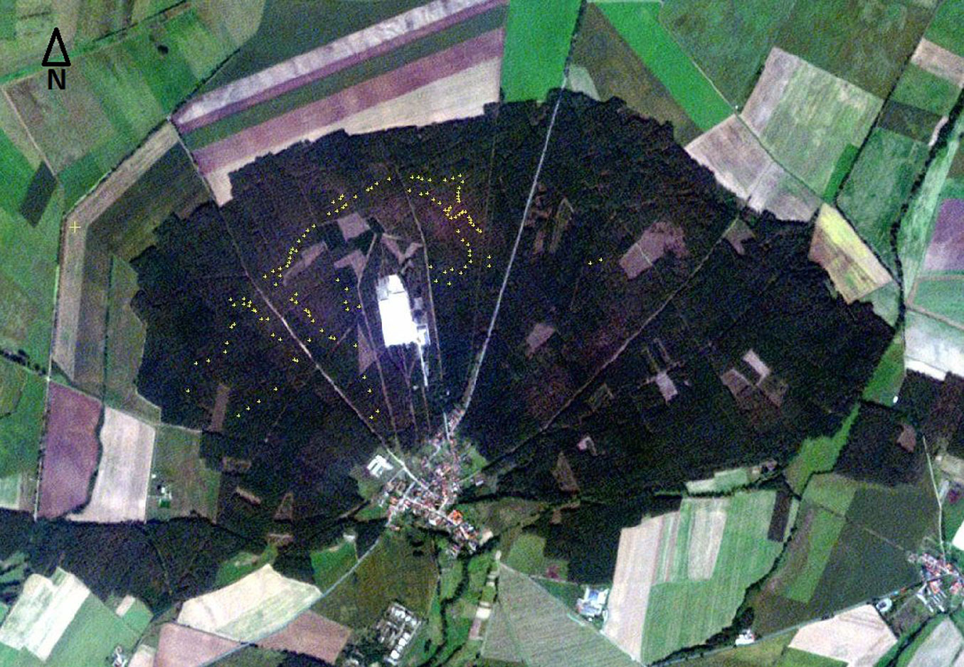
Ground reference samples required for the analysis of the statistical relationship between defoliation and the spectral variables were collected during the dates shown in Tab. 1. In test year 2012, the ground reference samples were dispersed over three RapidEye tiles, in 2013 and 2014 samples were covered by one tile. An expert of the state-forest research division carried out the foliage taxation of the Scots pine crowns using a standardized method of assessing PRF (percent remaining foliation). In practice, PRF is preferred above percent defoliation, because it indicates the survivability of a given tree, and because it is more intuitive. Sampling was performed on transects throughout the principal areas of infestation. Each sample point was selected in accordance with a relatively homogeneous condition of all pine crowns in the canopy within an estimated radius of about 10 m. The center coordinates of the sample points were recorded (Fig. 2) using a Magellan Mobile Mapper 6 equipped with ESRI ArcPad8 software. PRF was visually estimated for each tree in a plot in accordance with the state forest practice guide, using 11 possible PRF levels: 0%, 10%, 20%, 30%, 40%, 50%, 60%, 70%, 80%, 90%, and 100%. For each plot the average PRF value for all trees within was recorded. From the PRF levels, the memberships of the samples to the corresponding defoliation classes were determined. The defoliation classes are described in Tab. 2. The objective of the sampling strategy was to cover the entire range of occurring defoliation levels and to collect as many ground reference samples as possible in the given time. Although two reference photo books for defoliation estimation are available ([35], [4]), crown taxation based on photos from books or photos in general (Fig. 3A, Fig. 3B) may only provide guidance and orientation. A more reliable approach is illustrated in Fig. 4. It shows the method used to estimate the PRF-levels per tree and provides a calculation example. It is very helpful to divide the crown into sunlit and shaded crown and highly important to segment these parts regarding the yearly needle shoots, since it reduces the subjective error of visual impression. The attributes PRF and defoliation class were entered at the time of coordinate recording.
Fig. 2 - Example of GPS-measured sample plot centers (yellow crosses) over RapidEye RGB (test year 2014), 52° 17′ 27.0″ N 12° 12′ 02.0″ E, map scale: 1:50.000.
Tab. 2 - Defoliation classes derived from the 10 percent remaining foliation estimates (PRF).
| Defoliation class code | Description | Estimated PRF levels in defoliation class |
|---|---|---|
| c1 | none to minor defoliation | 90%, 100% |
| c2 | light to moderate defoliation | 80%, 70%, 60%, 50% |
| c3 | severe defoliation | 40%, 30%, 20% |
| c4 | extreme to complete defoliation | 10%, 0% |
Fig. 3 - Example of Scots pine trees with an estimated PRF (percent remaining foliage) value of: (a) 80%; and (b) 20% (photo: M. Wenk).
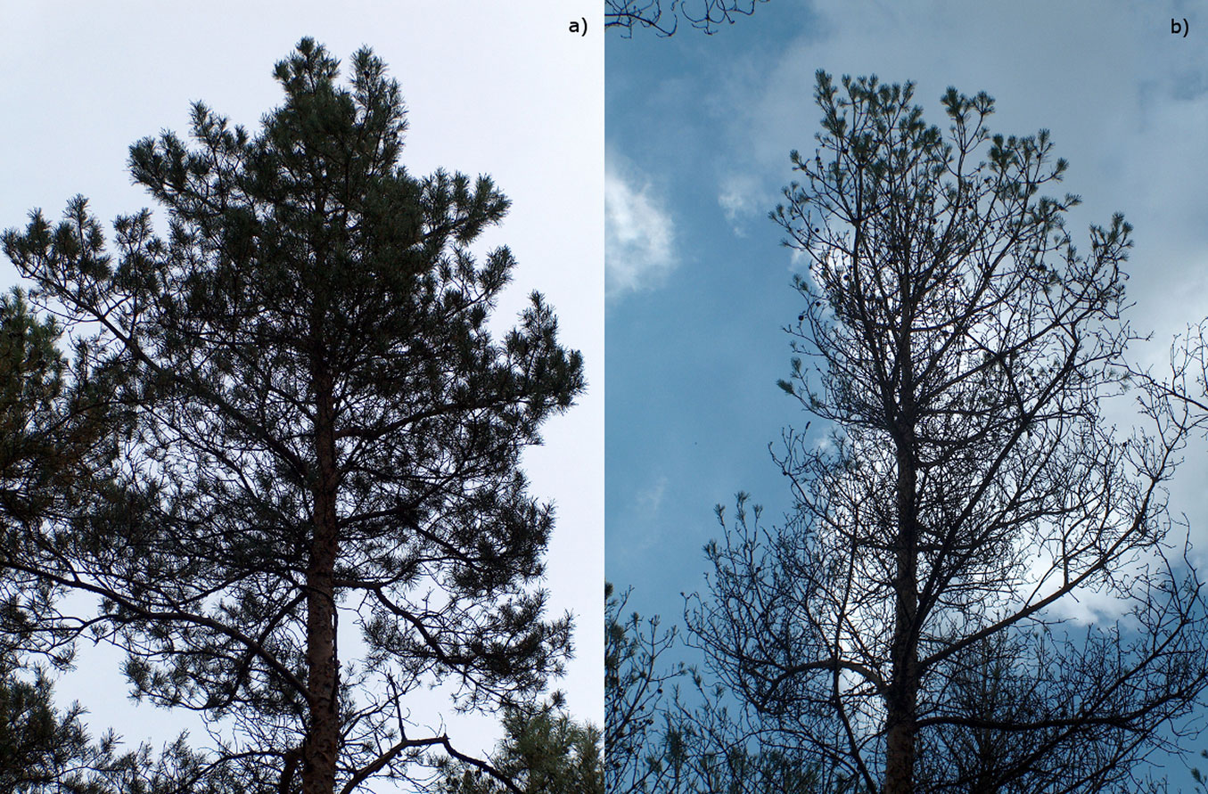
Fig. 4 - Method for the estimation of PRF levels for Scots pine (Eberswalde Forestry State Center of Excellence, Dept. Forest Development and Monitoring, Germany).
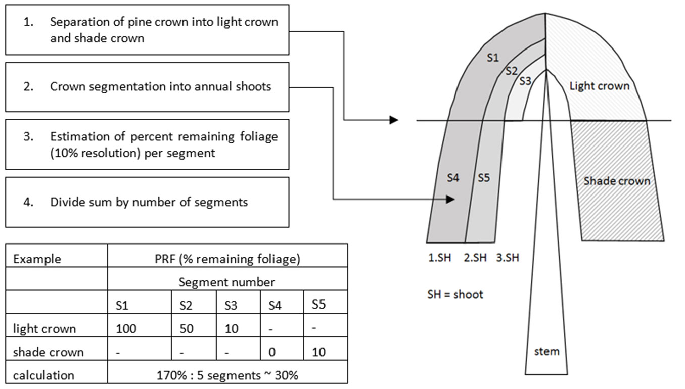
Image pre-processing and signature extraction
Pre-processing of the images included noise reduction based on the PCI maximum noise fraction linear transformation ([21]), and top of atmosphere correction ([8]). For the corrected images the vegetation indices NDVI [(NIR - red) / (NIR + red)] and NDRE [(NIR - red-edge) / (NIR + red-edge)] were calculated. A squared buffer of 10 m side lengths was applied to the sample points. The ground reference data were visualized with the images, and samples too close to forest roads and trails were discarded. Using the buffered samples image statistics (means of the five RapidEye bands, NDRE, and NDVI) were extracted using the EASI function VIMAGE in PCI Geomatics. The mean-function was used for signature extraction in order to average the spectral variability of the forest canopy within the sample plots. The attribute tables were exported to spreadsheets, and then imported to IBM SPSS for analysis.
Analysis of the relationship between the spectral variables and defoliation
The three test years were analyzed individually and not treated as one sample data set to avoid the introduction of additional error sources. Such error sources are for example varying time differences between image recording dates (IRD) and the dates of ground reference samples collection (GRD), the varying site conditions, and the different lighting conditions (sunny or cloudy) during sample collection. More details about such sources of uncertainty are reported in Eickenscheid & Wellbrock ([13]) and Muukkonen et al. ([36]).
The correlation analyses considered the whole range of PRF (0% to 100%). The Spearman’s ρ correlation coefficients ([34]) were calculated for all spectral bands, as well as for the NDRE and the NDVI, to assess the extent and direction of the relationships between the entire range of estimated PRF levels and the spectral variables.
To determine the capacity of the vegetation indices to distinguish between the four defoliation classes (Tab. 2), discriminant analyses (DA) were carried out for the three test years. As opposed to cluster analysis, which generates a grouping variable from feature variables, the DA explores the dependency of a nominally scaled grouping variable - in this study, the defoliation classes - to a metrically scaled feature variable (spectral variable). As DA requires normal distribution of the independent variable values within the groups of the dependent variable (defoliation classes), and equal group variances (homoscedasticity - [2]), normality of data was assessed using Shapiro Wilk’s tests, and equal variances using the Levene’s tests, both with α=0.05.
For the DA, the Wilk’s Lambda value is calculated by dividing the unexplained dispersion by the explained dispersion. Thus, the lower the Lambda value the higher the accuracy of the calculated discriminant function. The underlying H0 hypothesis expresses that the means of all independent variables are equal across the dependent variable’s groups. The significance of the Wilk’s Lambda values are tested by χ2 test (α=0.05). Significant χ2 values indicate that none of the independent variables is equal across groups of the dependent variable ([2]). For accuracy assessment, the leave-one-out cross validation method (LOO-CV) was selected. From the output results, classification confusion matrices were obtained and the corresponding producer’s (PA), user’s (UA), overall accuracies (OA), and KHAT-values were calculated. The KHAT value ranges between minus one and one and indicate if the actual agreement of the classification in the error matrix is significantly better than a random agreement ([11]). As a rule of thumb, KHAT > 0.75 indicates strong agreement, 0.5-0.75 represents moderate agreement, and KHAT < 0.5 a weak agreement ([32]). A negative KHAT value indicates that the classification result is worse than a random classification.
The ground reference data, the NDRE and the NDVI were used as input to a machine learning-based decision tree classifier (DTC). For this purpose, CRT (classification and regression trees, also known as CART or C&RT) of the IBM SPSS module Decision Trees was used. The underlying algorithm was developed and described in detail by Breiman et al. ([7]). When the dependent variable is categorical, CRT uses a recursive approach to generate a final classification tree, while a regression tree is created when the dependent variable is continuous. DTCs are non-parametric techniques which do not require Gaussian distribution or homoscedasticity of the independent variables ([53]). Therefore, individual classification trees could be generated for all three test years. CRT produces binary splits at each node of the decision tree based on user-defined criteria and creates child nodes and eventually end nodes (classes) in which the predictor variable is as homogenous as possible. The splitting criterion is defined as the deviation from the homogeneity and expressed in a measure of impurity ([28]). There are two impurity functions widely used in practice of which the GINI-Index is the most broadly used ([51]). The GINI impurity index reaches its minimum (zero) when all cases of an attribute fall into a single information class ([52]). Thus, the lower the GINI index is at a particular node the higher is the homogeneity of this node. Decision trees can become very complex since the algorithm tries to find a solution yielding the highest accuracy for the training data set. This will often result in too many tree levels and splits and sometimes solutions for single cases. There are several parameters which can be defined to create a more simplified and robust decision tree. The most important parameter for controlling the trade-off between robustness, accuracy and simplicity of the decision tree is pruning. Pruning reduces the complexity of the final decision tree and may result in a better predictive accuracy (robustness) by reducing the effect of overfitting and by removing sections that may be based on noisy or erroneous data ([37]). The intensity of pruning needs to be specified by the risk value (in the presented analyses set to 0.5) which defines the maximum acceptable risk difference between the unpruned and the pruned tree expressed in standard errors and ranges from zero (lowest risk) to one (highest risk - [28]). Other important parameters to be specified are the maximum number of tree levels (set to 3), the minimum number of cases for parent nodes (set to 10), and the minimum number of cases for child nodes (set to 5). Based on the set criteria, the decision tree grows during the learning process until the criteria are met. Then the tree is pruned back until the risk criterion is met. For the quality assessment of the final decision trees, a 10-fold cross validation was applied.
Results and discussion
Correlation analysis
The results of the correlation analysis (Tab. 3) showed that all spectral variables are sensitive to variations in tree foliage. The bands of the visible spectrum (i.e., the blue, green, red and red edge bands) were negatively correlated with PRF, proving the photosynthetic absorption characteristics mentioned above (see the introduction). Green and red-edge spectral wavelengths are absorbed by the chlorophyll pigments of green leaves with low specific absorption coefficients but simultaneously penetrate the leaves a little better than the main absorption bands blue and red. Thus, we can observe low to moderate correlations between the green and red-edge spectral wavelengths and PRF. In the case of the blue band the correlation analysis revealed low to moderate correlations with PRF. In contrast, the red band is the strongest correlating RapidEye band, even stronger than the NIR band. We assume that, apart from the chlorophyll component, the reddish-brown bark of Scots pine might be another coinciding and probably additive factor contributing to this effect. We also observed a negative correlation between the red band and PRF. When needle matter is lost due to insect feeding, less photosynthetically active needle mass is available (thus red increase) and at the same time the reddish bark becomes visible in the top view of the canopy (thereby red increase). The same observation was reported for Balsam fir by Lecki et al. ([31]) who attributed the increased red reflectance - next to the decreased chlorophyll absorption - to the higher reflectance of both bare twigs and feeding debris as compared to needles.
Tab. 3 - Spearman’s ρ correlation coefficients between spectral variables and estimated PRF-levels, ranking from 1 (highest overall correlation) to 7 (lowest overall correlation).
| PRF | Test year | N | Spearman’s ρ (PRF vs. spectral variables) |
||||||
|---|---|---|---|---|---|---|---|---|---|
| blue | green | red | red-edge | NIR | NDRE | NDVI | |||
| 0-100% | Test 1 (2012) | 95 | -0.55 | -0.56 | -0.69 | -0.43 | 0.70 | 0.88 | 0.85 |
| 0-100% | Test 2 (2013) | 203 | -0.77 | -0.69 | -0.89 | -0.73 | 0.83 | 0.90 | 0.90 |
| 0-100% | Test 3 (2014) | 122 | -0.28 | -0.46 | -0.80 | -0.37 | 0.75 | 0.85 | 0.86 |
| rank | - | - | 6 | 5 | 3 | 7 | 4 | 1 | 2 |
Positive correlations were observed between the NIR band and the vegetation indices. While the Spearman’s correlation coefficients of the blue, green, and red-edge band largely varied between the test years, they were more stable for the red band and for the NIR band and most stable for the vegetation indices. The correlations between PRF and the NDRE and NDVI were high, very similar, and approximately in the range of the observations made by Chávez & Clevers ([9]). The Spearman’s ρ of the three test years yielded the following ranking order (from highest to lowest overall correlation): NDRE, NDVI, red, NIR, green, blue, and red-edge.
Discriminant analysis
In test years 2012 and 2014 the statistical requirements for the DA (normality, homoscedasticity) were met, however, in the test year 2013 both vegetation indices showed significant departures from normality and homoscedasticity. Therefore, the test year 2013 had to be excluded from DA.
In the DA tests, all Wilk’s Lambda values were significant with an error probability p<0.001, as indicated by the Chi square test, i.e., the class means were not equal and the classes could therefore be separated. Detailed results of the discriminant analysis carried out including error matrices are shown in Tab. 4. The overall classification accuracy was moderate in test year 2012 (NDRE=70.5%, NDVI=70.5%) and relatively low in test year 2014 (NDRE=57.4%, NDVI=58.2%). Overall, considering the OAs and KHAT values, both vegetation indices perform nearly equally, as already observed in the correlation analysis. However, the detailed comparison of the defoliation classes UA’s and PA’s reveals the differences between the two vegetation indices. In defoliation class c2 and c4 the two vegetation indices perform similarly (see class coding in Tab. 2). In defoliation class c1 the NDRE performs visibly better than the NDVI by yielding on average a PA 12.4 percentage points higher and a UA 8.8 percentage points higher (see Tab. 5), i.e., the NDRE can better distinguish none to minor defoliation from moderate defoliation. In defoliation class c3 the NDVI exceeds the NDRE by 14.4 percentage points (PA) and 7.3 percentage points (UA). This suggests that the NDVI is more suitable to delineate severe defoliation from moderate defoliation.
Tab. 4 - Summary of the results of the discriminant analyses (DA) including error matrices. Combi refers to the combination of the NDVI and the NDRE in the DA. (χ2): Chi-square; (df): degrees of freedom; (PA): producer’s accuracy (%); (UA): user’s accuracy (%); (OA) overall accuracy (%).
| Test year 2012 | Test year 2014 | ||||||||||||||||
|---|---|---|---|---|---|---|---|---|---|---|---|---|---|---|---|---|---|
| Variable / Stats | class | Predicted | Σ | PA | Variable / Stats | class | Predicted | Σ | PA | ||||||||
| c1 | c2 | c3 | c4 | c1 | c2 | c3 | c4 | ||||||||||
| NDRE (OA=70.5 KHAT=0.59; Wilk’s λ=0.274; χ2=118.4; df=3; p-value = 0.000) |
Reference | c1 | 20 | 6 | 0 | 0 | 26 | 76.9 | NDRE (OA=57.4; KHAT=0.4; Wilk’s λ=0.305; χ2=140.7; df=3; p-value = 0.000) |
Reference | c1 | 11 | 4 | 0 | 0 | 15 | 73.3 |
| c2 | 5 | 25 | 4 | 0 | 34 | 73.5 | c2 | 16 | 24 | 12 | 0 | 52 | 46.2 | ||||
| c3 | 1 | 6 | 15 | 5 | 27 | 55.6 | c3 | 0 | 8 | 20 | 8 | 36 | 55.6 | ||||
| c4 | 0 | 0 | 1 | 7 | 8 | 87.5 | c4 | 0 | 0 | 4 | 15 | 19 | 78.9 | ||||
| - | Σ | 26 | 37 | 20 | 12 | 95 | - | - | Σ | 27 | 36 | 36 | 23 | 122 | - | ||
| - | UA | 76.9 | 67.6 | 75.0 | 58.3 | - | - | - | UA | 40.7 | 66.7 | 55.6 | 65.2 | - | - | ||
| NDVI (OA=70.5; KHAT=0.59; Wilk’s λ=0.277; χ2=117.5; df=3; p-value = 0.000) |
Reference | c1 | 17 | 9 | 0 | 0 | 26 | 65.4 | NDVI (OA=58.2; KHAT=0.43; Wilk’s λ=0.266; χ2=156.8; df=3; p-value = 0.000); |
Reference | c1 | 9 | 5 | 1 | 0 | 15 | 60.0 |
| c2 | 7 | 24 | 3 | 0 | 34 | 70.6 | c2 | 19 | 23 | 9 | 0 | 52 | 44.2 | ||||
| c3 | 1 | 2 | 19 | 5 | 27 | 70.4 | c3 | 0 | 6 | 25 | 5 | 36 | 69.4 | ||||
| c4 | 0 | 0 | 1 | 7 | 8 | 87.5 | c4 | 0 | 0 | 5 | 14 | 19 | 73.7 | ||||
| - | Σ | 25 | 35 | 23 | 12 | 95 | - | - | Σ | 28 | 34 | 40 | 19 | 122 | - | ||
| - | UA | 68.0 | 68.6 | 82.6 | 58.3 | - | - | - | UA | 32.1 | 67.6 | 62.5 | 73.7 | - | - | ||
| Combi (NDRE+NDVI) (OA=77.9; KHAT=0.69; Wilk’s λ=0.237; χ2=130.9; df=3; p-value = 0.000) |
Reference | c1 | 22 | 4 | 0 | 0 | 26 | 84.6 | Combi (NDRE+NDVI) (OA=65.6; KHAT=0.52; Wilk’s λ=0.231; χ2=173.4; df=3; p-value = 0.000) |
Reference | c1 | 11 | 3 | 1 | 0 | 15 | 73.3 |
| c2 | 5 | 26 | 3 | 0 | 34 | 76.5 | c2 | 12 | 28 | 12 | 0 | 52 | 53.8 | ||||
| c3 | 1 | 2 | 19 | 5 | 27 | 70.4 | c3 | 0 | 6 | 26 | 4 | 36 | 72.2 | ||||
| c4 | 0 | 0 | 1 | 7 | 8 | 87.5 | c4 | 0 | 0 | 4 | 15 | 19 | - | ||||
| - | Σ | 28 | 32 | 23 | 12 | 95 | - | - | Σ | 23 | 37 | 43 | 19 | 122 | - | ||
| - | UA | 78.6 | 81.3 | 82.6 | 58.3 | - | - | - | UA | 47.8 | 75.7 | 60.5 | 78.9 | - | - | ||
Tab. 5 - Average (test years 2012 and 2014) accuracy gains and losses in percentage points. Combi refers to the combination of the NDRE and NDVI in DA (discriminant analysis) and DTC (decision tree based classification). (Combi - NDRE/NDVI): accuracy gains (+) or losses (-) of the Combi over either vegetation index.
| NDRE vs. NDVI (DA) | NDRE or NDVI vs. Combi (DA) | DTC_Combi vs. DA_Combi | |||||||||
|---|---|---|---|---|---|---|---|---|---|---|---|
| PA gain | UA gain | OA gain | PA gain | UA gain | OA gain | PA gain | UA gain | OA gain | |||
| NDRE - NDVI | NDRE - NDVI | NDRE - NDVI | Combi - NDRE | Combi - NDVI | Combi - NDRE | Combi - NDVI | Combi - NDRE | Combi - NDVI | DTC-DA | DTC-DA | DTC-DA |
| 12.4 | 8.8 | -0.4 | 3.8 | 16.3 | 4.4 | 13.1 | 7.8 | 7.4 | -0.5 | 13.6 | 8.2 |
| 2.4 | -1.0 | - | 5.3 | 7.7 | 11.3 | 10.4 | - | - | 20.3 | 1.3 | - |
| -14.4 | -7.3 | - | 15.7 | 1.4 | 6.3 | -1.0 | - | - | -0.9 | 13.9 | - |
| 2.6 | -4.2 | - | 0.0 | 2.6 | 6.9 | 2.6 | - | - | 5.3 | 1.8 | - |
These results showed that, overall, neither of the two indices outperforms the other, exhibiting rather different performances in different defoliation classes. As a next step, the NDVI and NDRE were entered together (in combination) into the DA. The detailed results of this analysis are shown in Tab. 4. In classes c1, c2, and c3 the combination of the NDRE and NDVI fairly increased the classification accuracy, while the results of defoliation class c4 remained about the same. On average, the combination of the NDRE and NDVI in the test years 2012 and 2014 also increased the OA by 7.8 percentage points compared to the NDRE and 7.4 percentage points compared to the NDVI (Tab. 5).
Decision tree based classification
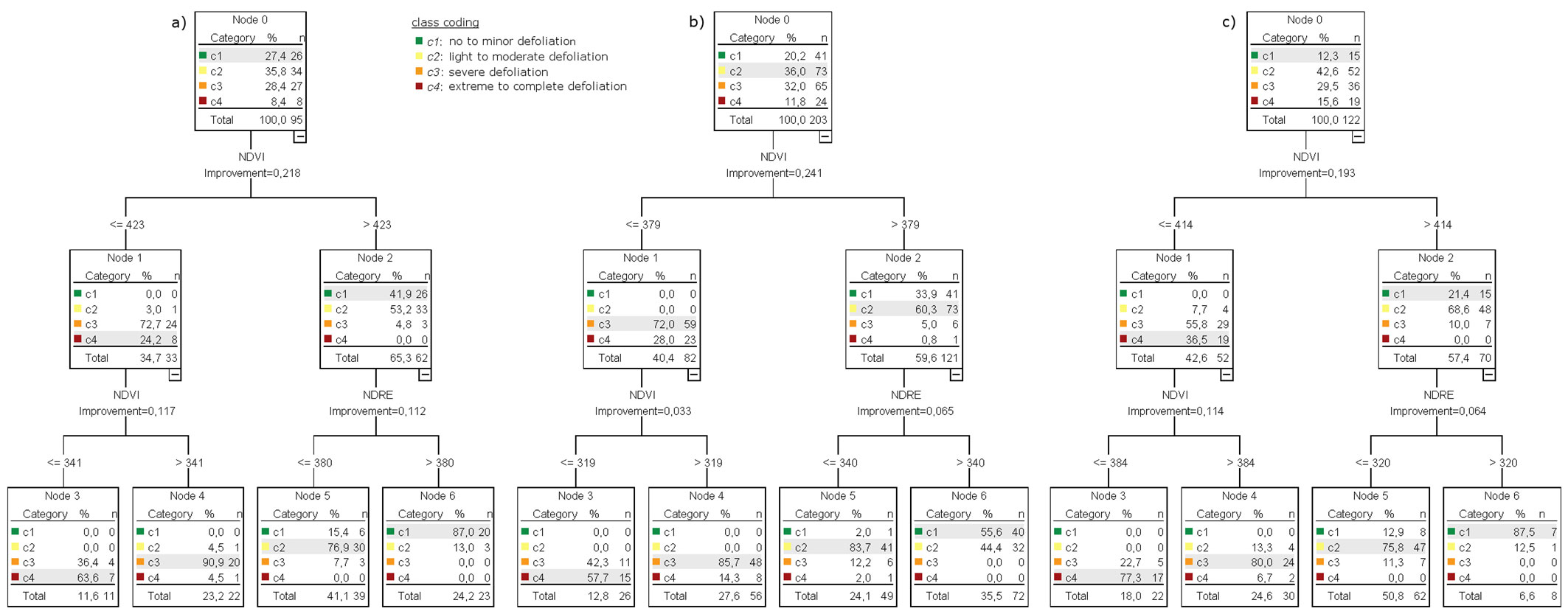
Tab. 6 summarizes the classification results achieved with the DTC. In all three models (compare Fig. 5a, Fig. 5b, Fig. 5c) the NDVI is selected for the first binary split producing the nodes one and two. The second binary split is also the same in the three models: node 1 used the NDVI to split into the two end nodes representing the defoliation classes c3 (node 3) and c4 (node 4), while node 2 used the NDRE to split it into the end nodes describing class c1 (node 5) and c2 (node 6). The use of the spectral indices by the classification tree displayed very similar pattern as observed in the correlation analysis and the DA, i.e., the NDRE better contributed to the detection of low defoliation levels (none to minor and moderate defoliation), whereas the NDVI better contributed to the detection of high defoliation levels (severe and extreme to complete defoliation). The resulting classification accuracies of the DTC are higher than those obtained by the DA using the NDRE and NDVI combination. For the test year 2012, the OA slightly increased from 77.9% to 81.1% (see Tab. 4 and Tab. 6), while we observed a strong OA enhancement of 13.1 percentage points for the test year 2014, mostly due to both user’s and the producer’s accuracy increases in the defoliation classes c1 and c2. Such increment in accuracy might be explained by a more skewed distribution of class data in the test year 2014 (as reflected by the lower p-values obtained in the normality test), which could lead to a bias in the DA results. In contrast, the non-parametric DTC could handle this data much better than the DA by creating a favorable tree structure. The comparisons of the average accuracy gains are shown in Tab. 5. The predictive power of the classification tree for test year 2013 was only moderate (OA=71%, KHAT=0.61).
Tab. 6 - Results and error matrices of the decision tree-based classifications (DTC) for the test years 2012, 2013, and 2014 using NDRE and NDVI as predictors (Combi). (PA): producer’s accuracy (%); (UA): user’s accuracy (%); (OA) overall accuracy (%).
| DTC_ Combi |
OA | KHAT | Predicted | ||||||
|---|---|---|---|---|---|---|---|---|---|
| class | c1 | c2 | c3 | c4 | Σ | PA | |||
| Test 1 (2012) | 81.1 | 0.73 | c1 | 20 | 6 | 0 | 0 | 26 | 76.9 |
| c2 | 3 | 30 | 1 | 0 | 34 | 88.2 | |||
| c3 | 0 | 3 | 20 | 4 | 27 | 74.1 | |||
| c4 | 0 | 0 | 1 | 7 | 8 | 87.5 | |||
| Σ | 23 | 39 | 22 | 11 | 95 | - | |||
| UA | 87 | 76.9 | 90.9 | 63.6 | - | - | |||
| Test 2 (2013) | 70.9 | 0.61 | c1 | 40 | 1 | 0 | 0 | 41 | 97.6 |
| c2 | 32 | 41 | 0 | 0 | 73 | 56.2 | |||
| c3 | 0 | 6 | 48 | 11 | 65 | 73.8 | |||
| c4 | 0 | 1 | 8 | 15 | 24 | 62.5 | |||
| Σ | 72 | 49 | 56 | 26 | 203 | - | |||
| UA | 55.6 | 83.7 | 85.7 | 57.7 | - | - | |||
| Test 3 (2014) | 78.7 | 0.7 | c1 | 12 | 3 | 0 | 0 | 15 | 80.0 |
| c2 | 5 | 43 | 4 | 0 | 52 | 82.7 | |||
| c3 | 1 | 6 | 24 | 5 | 36 | 66.7 | |||
| c4 | 0 | 0 | 2 | 17 | 19 | 89.5 | |||
| Σ | 18 | 52 | 30 | 22 | 122 | - | |||
| UA | 66.7 | 82.7 | 80.0 | 77.3 | - | - | |||
Fig. 5 - Final tree model for the PRF classification into four defoliation classes generated with CRT for (a) test year 2012, (b) test year 2013, and (c) test year 2014. Input variables: NDRE and NDVI.
Discussion of the trends observed in the classification results
Both the DA and the DTC classification showed similar classification pattern: the NDRE was more efficient in the detection of classes with none or moderate defoliation levels, whereas the NDVI works better for the classes representing severe or complete defoliation. Indeed, PRF is strongly correlated with both needle biomass and chlorophyll content, and it may be assumed that the NDRE responds better at high foliation levels because it does not saturate as quickly as the NDVI when the overall chlorophyll content of the forest canopy is high. This was observed by Eitel et al. ([14]), who tested in nursery of Scots pine seedlings the hypothesis that the additional availability of red-edge reflectance information would improve the detection of plant stress induced chlorophyll. The authors found that after removing the low chlorophyll values from the sample the spectral index chlorophyll relationship still amounted to r²=0.54 for the NDRE while it dropped to r²=0.34 for the NDVI.
Steele et al. ([47]) made very similar observations with grape leaves in a laboratory study based on chlorophyll (SPAD-502 device) and reflectance measurements (USB2000 radiometer). They suggested that the NDVI had a non-linear asymptotic relationship with chlorophyll and that its sensitivity decreased quickly when the chlorophyll content increased. In contrast, the NDRE showed a linear relationship, decreasing only slightly at high chlorophyll levels. Simultaneously, the slope of the NDVI fitting line became very steep at low chlorophyll levels - far steeper than the fitting line of the NDRE. This could explain a better response of the NDVI at low defoliation levels. Similar findings were reported by Viña et al. ([54]) who investigated the red-edge chlorophyll index [Chlred-edge= (NIR/ red-edge)-1] for its statistical relationship with green LAI in maize and soybean fields. Ritchie & Bednarz ([40]) investigated the relationship between the NDVI710nm (a red-edge based NDVI) and LAI estimates in cotton fields. The r² values calculated from this relationship at LAI < 0.5 equaled 0.87 and at LAI > 0.5 r² equaled 0.5. Obviously, in this study the observed differences between NDVI and NDRE could be due to specific changes in the chlorophyll content of the Scots pine canopy. To which extent leaf structure and chlorophyll content contribute to the specific NDVI and NDRE responses will be subject of further research.
Sources of uncertainty
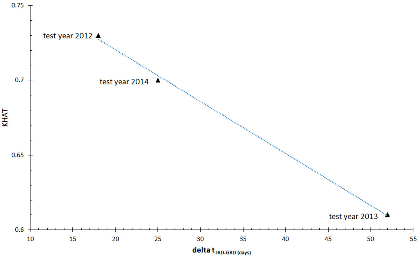
In this study, errors in the classifications obtained are probably due to the large lag time (Δt) between the image recording date (IRD) and the date of ground reference data collection (GRD). In fact, plotting the KHAT values of the classifications vs. Δt(IRD-GRD), a tight linear relationship was observed with decreasing KHAT values as the Δt increases (Fig. 6). In test year 2013 Δt(IRD-GRD) was the largest and amounts to 52 days (Tab. 1). In this year, the overall accuracy achieved with the DTC is the lowest. One of the consequences of the lag time is the increase in leaf area after the nun moth caterpillar activity has stopped. Pinus sylvestris is capable of growing new shoots and needles after severe defoliator attacks to compensate for the loss of foliage. This phenomenon has frequently been reported by foresters and we observed this also in the RapidEye imagery time series. Roloff ([41]) describes that in Scots pine the apical meristem at the base of the needle pairs is dormant under normal conditions; however, it is activated after defoliator damage or browsing damage. Within four weeks (A. Roloff, Technical University Dresden, Germany, pers. comm.) it will then start growing a new shoot with needles. The full regeneration process occurs at a scale of up to five years (depending on the damage where it begins) and its success depends on site conditions, climatic and biotic factors ([55], [56]).
Fig. 6 - Relationship between Δt (the lag time between image recording date - IRD, and the date of ground reference data collection - GRD) and KHAT values of decision tree-based classification.
Phenological changes of the understory vegetation are a further factor influencing the reflectance of the canopy. Moreover, another source of uncertainty was likely due to the sampling strategy adopted in this study, which could be biased as the samples were not selected at random. Finally, a varying degree of information in a pixel other than the defoliation may be attributed to the natural variability of the forest canopy (mixed pixels).
In insect defoliation studies, it has generally been asserted that a meaningful classification depth is limited to three defoliation classes yielding moderate overall accuracies between 70% and 80%, and that low defoliation levels remain difficult to detect ([39]). Taking the different sources of uncertainty into account, the results of our analysis confirmed this statement. However, we demonstrated that also low defoliation levels can be detected with moderate accuracy in Scots pine stands.
Conclusions and outlook
Based on the results of this study and previous literature evidence, we conclude that RapidEye is a suitable satellite-image data source for defoliation detection and mapping, as well as for general forest health mapping activities. The vegetation indices NDRE and NDVI are both well correlated with different levels of in situ estimated PRF. When the possibly early detection of defoliation is the objective, then the use of NDRE is the better option. Because of the sensitivity of NDRE to changes in chlorophyll content, it may also be used for other forest health problems associated with the symptomatic discoloration of needles, such as Armillaria root rot, epidemic infestations by bark or wood breeding insects (e.g., bark beetles and wood wasps), or in cases of anthropogenic effects such as massive sulfur dioxide emissions. If the objective is the precise delineation of severely or completely defoliated areas or other severe damages, then the use of NDVI has to be preferred. Using only one vegetation index can simplify processing procedures. When the objective is to produce maps with a maximum overall accuracy in all defoliation or otherwise defined damage classes, then a supervised method using both vegetation indices seems to be a meaningful approach, provided that a sufficient amount of ground-reference data of appropriate quantity and quality are available. Then, both the NDRE and NDVI can be combined and used for instance in a decision tree classifier such as CART, Ross Quinlan’s C5, or a Random Forest classifier.
Future research should be addressed to better understand the defoliation and re-foliation processes from the early symptoms until the full regeneration or death of affected pine stands by analyzing RapidEye time series of known defoliation hotspots. In this context, a variety of influencing factors (e.g., climatic variables, stand and site parameters such as age, density, type of understory vegetation, soil type, and forest management practices) could be included in the analysis, with the aim of better understanding the defoliator gradation cycles, revealing patterns of geo-spatial spreading of insect populations or even developing appropriate prediction models. Furthermore, the inclusion of defoliator infested stands with and without pesticide treatment would also be of great interest, as it could bolster ecologically and economically more sustainable forest health management.
Acknowledgements
We thank Matthias Wenk from the Eberswalde Forestry State Center of Excellence, Dept. Forest Development and Monitoring, Germany, whose expertise in pine crown foliage taxation is acknowledged. We also thank all the foresters for the interesting discussions and their support, and Dr. Katrin Möller from the Eberswalde Forestry State Center of Excellence for her support. Finally, we thank Lauren Jean Roerick and Pablo Rosso for revising the English language, and the Planet Labs for this interesting research opportunity.
References
Gscholar
Gscholar
Gscholar
Gscholar
Gscholar
Online | Gscholar
Online | Gscholar
Gscholar
Gscholar
Gscholar
Gscholar
Gscholar
Gscholar
Online | Gscholar
Gscholar
Online | Gscholar
Gscholar
Authors’ Info
Authors’ Affiliation
Planet Labs Germany GmbH, Kurfürstendamm 22, D-10719 Berlin (Germany)
Technische Universität Berlin, Geoinformation in Environmental Planning Lab, Straße des 17.Juni 145, D-10623 Berlin (Germany)
Corresponding author
Paper Info
Citation
Marx A, Kleinschmit B (2017). Sensitivity analysis of RapidEye spectral bands and derived vegetation indices for insect defoliation detection in pure Scots pine stands. iForest 10: 659-668. - doi: 10.3832/ifor1727-010
Academic Editor
Alessandro Montaghi
Paper history
Received: Jun 02, 2015
Accepted: May 04, 2017
First online: Jul 11, 2017
Publication Date: Aug 31, 2017
Publication Time: 2.27 months
Copyright Information
© SISEF - The Italian Society of Silviculture and Forest Ecology 2017
Open Access
This article is distributed under the terms of the Creative Commons Attribution-Non Commercial 4.0 International (https://creativecommons.org/licenses/by-nc/4.0/), which permits unrestricted use, distribution, and reproduction in any medium, provided you give appropriate credit to the original author(s) and the source, provide a link to the Creative Commons license, and indicate if changes were made.

Web Metrics
Breakdown by View Type
Article Usage
Total Article Views: 41398
(from publication date up to now)
Breakdown by View Type
HTML Page Views: 34478
Abstract Page Views: 2154
PDF Downloads: 3932
Citation/Reference Downloads: 45
XML Downloads: 789
Web Metrics
Days since publication: 2473
Overall contacts: 41398
Avg. contacts per week: 117.18
Article Citations
Article citations are based on data periodically collected from the Clarivate Web of Science web site
(last update: Feb 2023)
Total number of cites (since 2017): 17
Average cites per year: 2.43
Publication Metrics
by Dimensions ©
Articles citing this article
List of the papers citing this article based on CrossRef Cited-by.
Related Contents
iForest Similar Articles
Review Papers
Accuracy of determining specific parameters of the urban forest using remote sensing
vol. 12, pp. 498-510 (online: 02 December 2019)
Research Articles
Remote sensing of Japanese beech forest decline using an improved Temperature Vegetation Dryness Index (iTVDI)
vol. 4, pp. 195-199 (online: 03 November 2011)
Review Papers
Remote sensing-supported vegetation parameters for regional climate models: a brief review
vol. 3, pp. 98-101 (online: 15 July 2010)
Technical Reports
Detecting tree water deficit by very low altitude remote sensing
vol. 10, pp. 215-219 (online: 11 February 2017)
Review Papers
Remote sensing of selective logging in tropical forests: current state and future directions
vol. 13, pp. 286-300 (online: 10 July 2020)
Research Articles
Development of monitoring methods for Hemlock Woolly Adelgid induced tree mortality within a Southern Appalachian landscape with inhibited access
vol. 9, pp. 178-186 (online: 02 January 2016)
Research Articles
Influence of climate on tree health evaluated by defoliation in the ICP level I network (Romania)
vol. 10, pp. 554-560 (online: 05 May 2017)
Research Articles
Afforestation monitoring through automatic analysis of 36-years Landsat Best Available Composites
vol. 15, pp. 220-228 (online: 12 July 2022)
Technical Reports
Remote sensing of american maple in alluvial forests: a case study in an island complex of the Loire valley (France)
vol. 13, pp. 409-416 (online: 16 September 2020)
Research Articles
Assessing water quality by remote sensing in small lakes: the case study of Monticchio lakes in southern Italy
vol. 2, pp. 154-161 (online: 30 July 2009)
iForest Database Search
Search By Author
Search By Keyword
Google Scholar Search
Citing Articles
Search By Author
Search By Keywords
PubMed Search
Search By Author
Search By Keyword


