On the exposure of hemispherical photographs in forests
iForest - Biogeosciences and Forestry, Volume 6, Issue 4, Pages 228-237 (2013)
doi: https://doi.org/10.3832/ifor0957-006
Published: Jun 13, 2013 - Copyright © 2013 SISEF
Research Articles
Abstract
At least 10 different methods to determine exposure for hemispherical photographs were used by scientists in the last two decades, severely hampering comparability among studies. Here, an overview of the applied methods is reported. For the standardization of photographic exposure, a time-consuming reference measurement in the open land towards the unobstructed sky was required so far. The two Histogram Methods proposed here make use of the technical advances of digital cameras which enable users to assess a photograph’s histogram directly at the location of measurement. This avoids errors occurring due to variations in sky lighting happening in the time span between taking the reference measurement and reaching the sample location within the forest. The Histogram Methods speed up and simplify taking hemispherical photographs, and introduce an objectively applicable, standardized approach. We highlight the importance of correct exposure by quantifying the overestimation of gap fraction resulting from auto-exposed photographs under a wide range of canopy openness situations. In our study, gap fraction derived from auto-exposed photographs reached values up to 900% higher than those derived from non-overexposed photographs. By investigating the size of the largest gap per photograph and the number of small gaps (gaps contributing less than 0.1% to gap fraction), we concluded that the overestimation of gap fraction resulted mainly from the overexposure of vegetation surrounding large gaps.
Keywords
Introduction
Solar radiation is the ultimate source of energy for life and a major determinant of the physiology, morphology, behavior, and life history of most organisms ([35]). To assess light conditions in forest stands hemispherical photography is a widely used non-destructive observation technique ([20]). Using a fisheye lens with a field of view of 180° pointing upwards from below the canopy, photographs are rapidly acquired in the field and provide users with a permanent high resolution documentation of the current geometry of canopy openings ([57]). Gap fraction, defined as the proportion of sky pixels in the photograph, is the basic measurement of hemispherical photographs ([31]). Moreover, the effective leaf area index (eLAI), a critical structural parameter required in ecological and process-based canopy photosynthesis models, is estimated based on the obstruction/penetration pattern of vegetation ([80]). Foliage distribution and leaf angle distribution ([57]), radiation microclimate below canopies ([69], [77]), annual near-ground solar radiation ([82]), and horizontal and vertical heterogeneity in canopies ([48]) are also derived from hemispherical photographs. Hemispherical photographs are also used in calibration studies for terrestrial and airborne laser scanning ([12], [43], [58], [62]).
Hemispherical photography is a multi-step process prone to errors at each step ([57]). Errors may arise from: (1) camera positioning and orientation; (2) photographic exposure; and (3) selection of a threshold to distinguish foliage from canopy openings, the so called “thresholding“ ([57]).
Considering these errors, Wagner ([74]) emphasized that radiation values determined for the purpose of comparing different sites are only of interest if measurements are reproducible. Comparability is, however, often hampered due to missing standard protocols for acquisition and analysis of hemispherical photographs ([57], [74], [80]).
Usually, camera positioning is 1.2 meters above ground level facing exactly vertical. Standardization of the thresholding can be achieved by applying an automated thresholding procedure as recommended by several authors ([31], [45]). The standardization of photographic exposure is challenging as exposure settings need to account for differences in luminance between scenes caused by differences in weather conditions, degree of cloudiness, and solar altitude. At the same time, exposure should allow for a good separation of sky and vegetation pixels in the resulting photograph.
Various studies have been published over the past decades on how to standardize exposure in hemispherical photography ([8], [73], [74], [80]). It was found that if exposure is too low, that is, the resulting photographs are too dark, grey values of sky and vegetation pixels become too similar to be separated. If exposure is too high, that is, the resulting photographs are too bright, vegetation which is bordering canopy gaps is overexposed, and thus, gaps appear larger than they really are ([57], [80]). In consequence, estimates of gap fraction derived from differently exposed photographs may differ substantially (e.g., [50], [73], [80]).
Taking standardized photographs in the field requires a reference measurement taken in the open land by aiming an external exposure meter (angle of view lower than 10°) at the brightest spot in the scene, i.e., the sky. For the subsequent photograph taken within the forest, exposure has to be increased by 2-3 exposure values (EV) relative to this reference measurement ([74]). Using the above procedure, the photograph is exposed for the brightest spot in the scene, hence avoiding overexposure, while the full dynamic range of the camera’s sensor is used. In photography, a change of ± 1 EV represents a doubling or halving of the amount of light reaching the camera sensor. Therefore, to make an unobscured sky (18% visible reflectivity) appear completely white (100% visible reflectivity) theoretically 2.5 EVs of overexposure are required ([39]).
Although Chen et al. ([8]), Wagner ([74]), and Zhang et al. ([80]) have provided a theoretical basis for standardizing exposure in hemispherical photography, a number of unstandardized methods for determining exposure continues to be used by many in the scientific community.
In the present study, a literature review was compiled to identify existing methods for the determination of the exposure of hemispherical photographs. By analyzing the grey value histograms of differently exposed photographs we illustrate the influence of the exposure determination method on a photograph’s grey values. Further, we present two protocols by which the correct exposure can be rapidly determined in the field. To highlight the importance of a standardized method to determine exposure in hemispherical photography, we compare gap fraction estimates derived from auto-exposed photographs to those derived from correctly exposed photographs. The errors arising from auto-exposure are quantified for a NIKON® D70s DSLR for a wide range of canopy openness situations found in subtropical ecosystems in southern China.
Literature review
We analyzed 61 publications appeared between 1991 and 2012 in which hemispherical photography was applied and identified ten different exposure determination methods (Tab. 1). The most frequently used method was the auto-exposure which leaves the decision on how to expose the photograph completely to the camera’s software (e.g., [66], [27]). Beaudet & Messier ([3]) apply the bracketing function of the camera to shoot a series of differently exposed photographs and manually select the photograph showing the best contrast between sky and vegetation for further analysis. Stohr & Bilhimer ([64]) propose using image processing software such as Adobe Photoshop Elements© to correct poor photographs in which the solar disc appears or which have little contrast between sky pixels and vegetation pixels. Matsuyama et al. (2003, cited in [79]) recommend taking a reference measurement outside the forest using a built-in camera light meter and to use the same exposure for taking photographs within the forest. Chen et al. ([8]) suggest overexposing the photograph by 1-2 EV compared to a reference measurement outside the forest. Finally, some authors say virtually nothing on the used exposure settings at all (e.g., [9], [48]).
Tab. 1 - Exposure determination methods found in 61 publications using hemispherical photography.
| Exposure determination method | Number of publications | Found in |
|---|---|---|
| Auto-exposure | 13 | [2], [10], [13], [16], [19], [21], [24], [25], [26], [27], [31], [49], [66] |
| Bracketing (auto-exposure, -1, -2 EVs or auto-exposure, +2, -2EVs) and selection of “best” photograph | 5 | [3], [20], [36], [38], [46] |
| Underexposed by -2 EVs to reference within forest | 1 | [32] |
| Underexposed by -1 EV to reference within forest | 1 | [56] |
| Underexposed by -0.7 EVs to reference within forest | 1 | [29] |
| Overexposed by 2-3 EVs to reference in open land |
11 | [4], [11], [68], [40], [58], [71], [72], [73], [74], [75], [80] |
| Overexposed by 1-2 EVs to reference in open land |
3 | [8], [30], [62] |
| Overexposed by 1 EV to reference in open land |
2 | [47], [61] |
| Same exposure as reference in open land | 3 | [28], Matsuyama et al. 2003 (in [79]), [79] |
| Posterior correction of photographs using image manipulation software |
1 | [64] |
| No statement | 20 | [1], [5], [9], [12], [22], [23], [33], [34], [37], [41], [43], [45], [48], [52], [54], [55], [60], [69], [70], [81] |
Excursus: photography technique
Dynamic range and exposure
A scene’s dynamic range is defined as the ratio of the maximum light intensity (brightest spot) to the minimum light intensity (darkest spot) in the scene ([14]). By analogy, the range of light intensities which can be recorded by a camera sensor is defined as the ratio of maximum light intensity measurable to the minimum light intensity measurable ([53]).
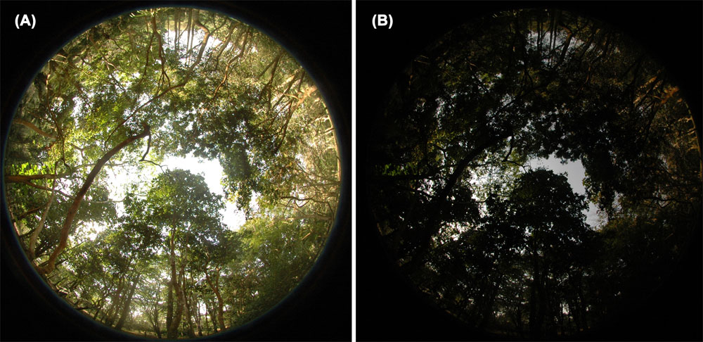
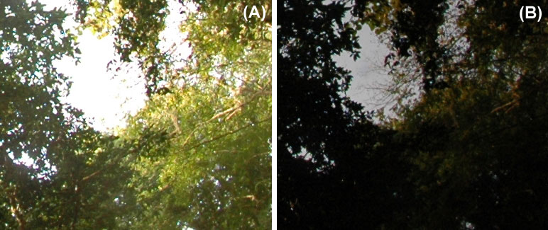
When capturing a scene which contains a dynamic range that exceeds that of the camera, a loss of detail occurs either in the lowlight areas, the highlight areas, or both ([59]). This is a common problem in photography since digital cameras have a dynamic range that is often lower than that encountered in the real world ([42]). Hemispherical photography suffers particularly from the limited dynamic range of camera sensors since forest scenes photographed from below the canopy towards the zenith have a very high dynamic range resulting from dark understory vegetation and bright sky coming into view simultaneously (Fig. 1a, Fig. 1b).
Fig. 1 - (A) Auto-exposed photograph taken with aperture F6.7 and shutter speed 1/125s. Gap fraction: 8.83%; number of gaps: 5848; LGI: 2.19%. (B) Non-overexposed photograph (underexposed by -3.5 EVs) taken at the same location. Aperture F11 and shutter speed 1/500s. Gap fraction: 1.78%; no. of gaps: 1177; LGI: 1.23%. Resolution of circular image area: 1 998 029 pixels.
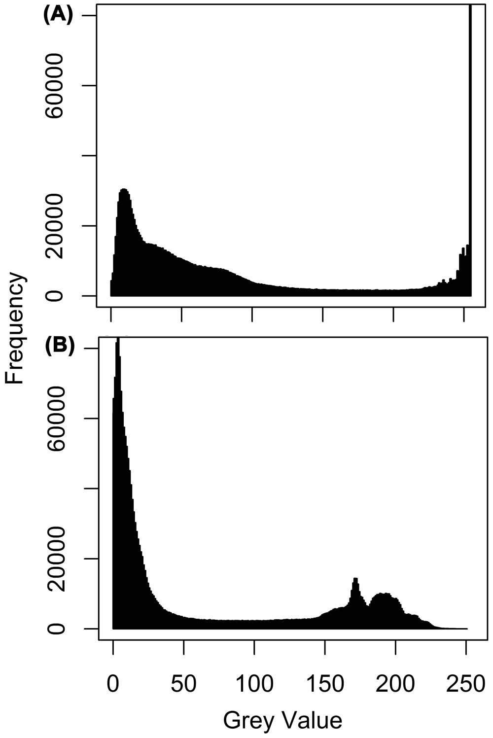
The grey value histogram of a photograph can be used very effectively to assess a possible mismatch between a scene’s and a camera’s dynamic range. Only when frequencies of grey values decrease towards both ends of the histogram’s x-axis, the dynamic range of a scene is completely covered. Frequency bins grouped against the extreme left end of the histogram indicate underexposure or blocked up shadows, which are areas of pure black (Fig. 2b). Frequency bins grouped against the extreme right end of the histogram indicate overexposure or blown highlights, which are areas of pure white (Fig. 2a). In these over-or underexposed parts of the photograph a reliable differentiation of sky and vegetation pixels is impossible.
Fig. 2 - (A) Grey value histogram of an auto-exposed photograph. The bright end of the dynamic range is cut off due to overexposure. This is indicated by the peak at the right end of the histogram. (B) Grey value histogram of a non-overexposed photograph. The dark end of the dynamic range is cut off.
Via photographic exposure one can control which section of a scene’s dynamic range is captured in the photograph. Exposure is defined as the total density of light (measured in lux seconds) allowed falling onto the sensor; it is controlled by the settings for shutter speed and lens aperture. Changing these settings while accounting for the sensor’s sensitivity (ISO), the user can control which light levels will be captured, and which light levels will be lost due to saturation of the camera’s dynamic range ([59]).
Automatic exposure
Common camera light meters assume the scene to be photographed as a mid-grey surface which reflects 18% of incident light ([67]). Thus, the camera’s auto-exposure adjusts aperture width and shutter speed accordingly to produce a photograph which has an average grey value of 18% as well. This “18% neutral grey standard” satisfies most photographers because it allows the camera’s light meter to render correct readings for average scenes in average lighting situations.
With hemispherical photography, auto-exposure has the effect that the more vegetation covers, thus darkens the scene, the higher is the exposure set by the camera. For dark scenes, this results in photographs in which the forest interior is colorful depicted but the sky and as well brightly illuminated vegetation parts are overexposed and appear completely white (Fig. 1a). In contrast, for bright scenes with low proportions of vegetation, the sky is displayed in detail, but color information on vegetation is lost (Fig. 1b). Hemispherical photographs taken in forests are dominated by vegetation, and therefore, mainly affected by the loss of information due to overexposure.
For exposure, DSLRs offer the possibility to choose between different metering modes to determine a scene’s luminance, for example, spot, center-weighted, and matrix metering in NIKON’s D70s. Spot metering measurements are made from a circular spot (2.3 mm diameter) which are averaged for exposure determination. Bright or dark areas within the spot will give extreme readings ([44]). Center-weighted metering averages the circular area (8 mm diameter) in the middle of the frame and gives that calculation a 75% weight in the overall computation for exposure ([44]). Nikon’s matrix meter gathers information using a 1005-pixel RGB CCD sensor as it evaluates exposure. Other camera manufacturers offer similar exposure metering modes which differ in their specifications, e.g., partial metering (approx. 6.5% of viewfinder at center), spot metering (approx. 2.8% of viewfinder at center), and center-weighted average metering in CANON’s EOS 60D ([6]).
Optimal exposure of hemispherical photographs
The first step in processing hemispherical photographs is the photograph’s binarization ([31]). By setting a threshold on the photograph’s grey values, vegetation pixels are separated from sky pixels. Based on the binarized photograph, stand characteristics are modeled by computer programs like, e.g., Gap Light Analyzer 2.0 ([17]), Winscanopt (Regent Instruments Inc., Quebec, Canada), HemiView v8 (Delta-T Devices Ltd. 1999), and CAN-EYE v6.1 ([76]). It is worth noting that all modeling is exclusively based on the binarized image; color information is not accounted for. In hemispherical photography it is therefore not required to expose photographs such that the forest interior is rendered in great detail. Rather, exposure should aim at the correct and sharp depiction of canopy openings. At the same time the full dynamic range of the camera’s sensor should be used so that contrast between sky and vegetation is maximized, thus, allowing for a good separability of sky and vegetation pixels. These two criteria can be fulfilled through exposing the photograph for the scene’s brightest spot. This can be approached by the above described procedure by Wagner ([74]) which achieves this by relating exposure to a reference measurement taken outside the forest. Since new DSLRs allow for an immediate analysis of the photograph’s histogram, the two Histogram Methods (as described in the next chapter) can be applied as well. All three methods prevent overexposure by pushing the grey value of the brightest spot in a scene close to, but not up against, the right edge of the photograph’s grey value histogram.
Exposure determination using photograph histograms
The proposed Histogram Methods require that at each sample location a series of photographs is shot. After each shot, it needs to be assessed whether the photograph is affected by overexposure. If so, exposure needs to be decreased. This can be easily done in steps of 1/2 or 1/3 EV by using the camera’s exposure compensation function.
The following two approaches can be applied to prevent overexposure while maximizing contrast in the photograph:
- Take a hemispherical photograph of a chosen site. Assess the photograph’s histogram via the camera’s display mode. If the histogram shows a saturation/peak at the very right end of the x-axis, exposure needs to be decreased until the peak disappears. If the frequency bins of the histogram do not reach the right end of the x-axis, exposure has to be increased until they almost do.
- Take a hemispherical photograph of a chosen site. Review the photograph using the camera’s “highlight clipping warning” (Nikon) or “highlight alert“ (Canon) playback mode. In this playback mode all overexposed areas are marked as blinking lights which show the spatial distribution of the rightmost frequency bin in the corresponding grey value histogram. Exposure has to be decreased until the warning lights disappear. If no warning lights appear, exposure has to be increased towards one step below that exposure at which the warning lights appear.
Methods
Study site
Data were collected in Xishuangbanna Tropical Botanical Garden (XTBG - WGS 84: 21°55’39.36” N 101°15’51.84” E) which is located in Xishuangbanna, Yunnan, China. The wide range of canopy openness situations found in the botanical garden provided us with ideal conditions to assess the characteristics of gap fraction estimates derived from hemispherical photographs. Photographs were taken at 97 locations in the botanical garden aiming at covering a wide range of canopy openness situations.
Photograph acquisition
A Nikon D70s DSLR equipped with a Sigma Circular Fisheye 4.5mm 1:2.8 lens with a field of view of 180° was used. The camera was mounted on a tripod at 1.2m height to characterize the canopy without the interfering presence of understory vegetation ([65]). The camera was leveled to face exactly the vertical using a bubble-level slotted into the flash socket. The top of the camera (position of the flash socket) was orientated to magnetic north using a compass ([3]). Photographs were taken without direct sunlight entering the lens ([56]) in the early morning, late afternoon, or on overcast days ([78]).
The basic camera settings mode “P” (Programmed Auto), ISO = 400, and matrix metering were used. At each location an auto-exposed photograph was taken. Subsequently EV was reduced in steps of 1/2 EV until the photograph’s grey value histogram and the “highlight clipping warning” function of the camera indicated that no overexposed pixels were left in the photograph (Histogram Methods a and b). At each EV level, one photograph was taken. Photographs were stored in JPEG format (3008 × 2000 pixels resolution), since no difference in grey values between TIFF and JPEG format was found ([18]).
Photograph processing and analysis
All processing and analysis was done using R ([51]) and the EBImage package ([63]). The blue color planes of the 8-bit RGB hemispherical photographs were selected for the analysis. Best separability of sky and vegetation pixels in the blue color plane results from skies tending to scatter blue light and low scattering of blue light by leaves ([7], [36]). To remove the black frame surrounding the photograph of interest the blue color plane was clipped with a mask file setting all pixel values outside the central circular area to “n/a” (not available).
An automated global thresholding was applied to avoid variations in threshold setting by manual interpretation of photographs and because it speeded up the processing time ([15], [30]). The thresholding algorithm iteratively calculated grey value histograms with subsequently increasing bin width. As soon as the histogram showed exactly one minimum between two modes, the threshold was defined as the middle of this minimum bin. Each pixel with a grey value equal or below that threshold was classified as vegetation; all pixels with a grey value above were classified as sky.
For each location gap fraction values were derived from: (1) the auto-exposed photograph, and (2) the non-overexposed photograph, resulting from the application of the Histogram Methods. Besides comparing the paired gap fraction values, as well the number of gaps and the largest gap index (LGI) derived from the auto-exposed and the non-overexposed photograph were compared. We defined the LGI as the proportion of the photograph covered by the largest gap.
Photographs were post stratified into stratum “open” (gap fraction > 30%, N=16), “medium” (gap fraction 15-30%, N=8), and “dense” (gap fraction < 15%, N=73). As well figures were analyzed over all strata (gap fraction 0-50%, N=97). Pairs of images were tested with the paired Wilcoxon signed rank test for statistically significant differences; all p-values given refer to this test at the 0.05 alpha level.
Results
Exposure
Visual examination of photographs taken within forests revealed that auto-exposed photographs appeared brighter and contained a wider range of green and brown tones than non-overexposed photographs. Fig. 1a, Fig. 1b and Fig. 2a, Fig. 2b show photographs and histograms taken at one location. The histogram of the auto-exposed photograph shows a peak at grey value 255 indicating overexposure and a loss of information in the bright areas of the photograph (Fig. 2a). In the histogram of the non-overexposed photograph, frequency bins gradually decreased towards the right end of the x-axis, indicating that no information was lost in the bright components of the photograph (Fig. 2b). Instead, a peak at the left end of the x-axis occurred indicating a slight loss of color information in the dark areas due to underexposure.
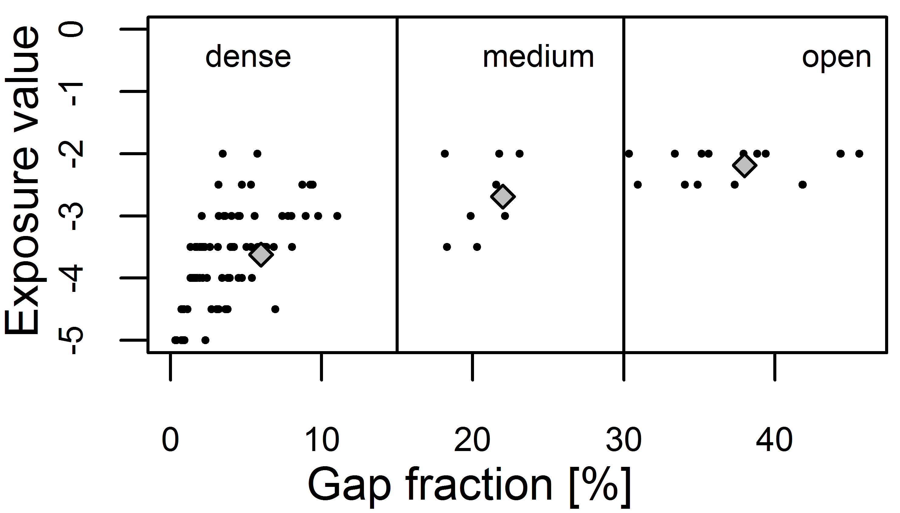
On average, photographs had to be underexposed by -3.3 EVs to avoid overexposure. We observed that more underexposure was required under dense canopy conditions than under open canopy conditions (Fig. 3). Post stratified data showed that the on-average required underexposure increased from stratum “open” (-2.2 EVs), via “medium” (-2.7 EVs) to “dense” (-3.6 EVs). While in all strata the minimum required underexposure was -2 EVs, the maximum required under exposure increased from -2.5 EVs in stratum “open”, via -3.5 EVs in “medium” to -5 EVs in “dense”.
Fig. 3 - Scatterplot of gap fraction [%] as measured in non-overexposed photographs against the exposure value required to avoid overexposure. Photographs taken under dense canopy conditions require more steps of underexposure than photographs taken under open canopy conditions. Grey diamonds: per stratum.
Gap fraction estimates
Gap fraction estimates derived from non-overexposed photographs ranged from 0.32 to 45.59%. Estimates based on auto-exposed photographs covered a slightly different range from 3.2 to 49.97% (Tab. 2, Fig. 4). The average difference between gap fraction estimates was 6.18% and medians calculated over all strata differed significantly between the auto-exposed and non-overexposed photographs (p <0.001).
Tab. 2 - Mean (standard deviation in parenthesis) and median of gap fraction estimates [%] derived from non-overexposed and auto-exposed photographs. And mean and median of relative differences of gap fraction estimates [%] between non-overexposed and auto-exposed photographs.
| Stratum | non-overexposed | auto-exposed | relative difference | |||
|---|---|---|---|---|---|---|
| Mean | Median | Mean | Median | Mean | Median | |
| all | 10.96 (13.19) |
4.6 | 17.16 (11.34) |
12.83 | 56.32 | 152.61 |
| open | 37.87 (4.76) |
37.63 | 39.62 (5.09) |
40.15 | 4.64 | 2.35 |
| medium | 20.65 (1.8) |
20.93 | 25.29 (4.02) |
25.07 | 22.44 | 22.37 |
| dense | 4.02 (2.6) |
3.62 | 11.35 (3.25) |
11.27 | 181.96 | 208.01 |
Fig. 4 - Box-plots of gapm non-overexposed and auto-exposed photographs. Box: first, second, and third quartile; whiskers: 1.5 x interquartile range; grey diamonds: mean gap fraction.
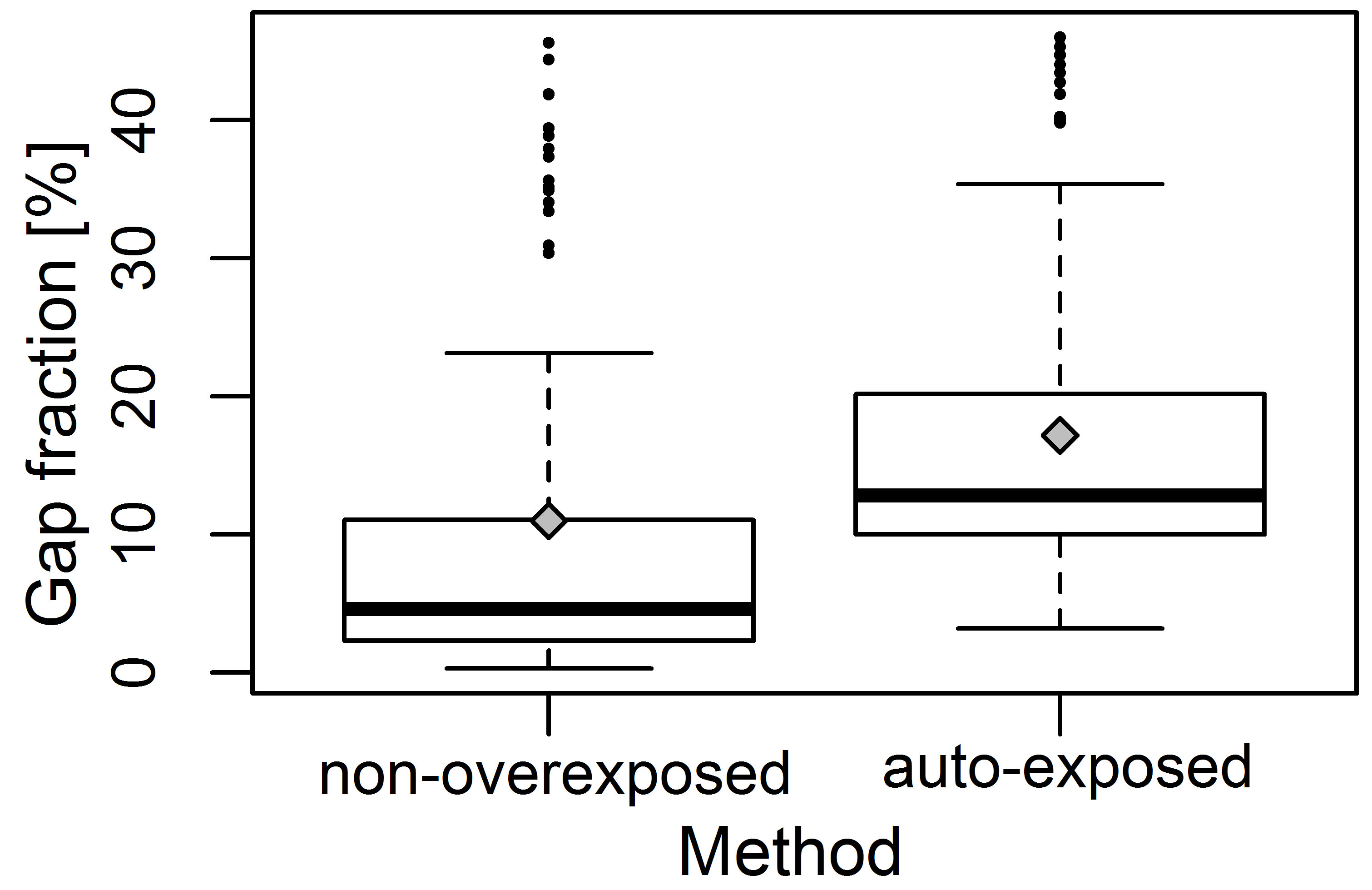
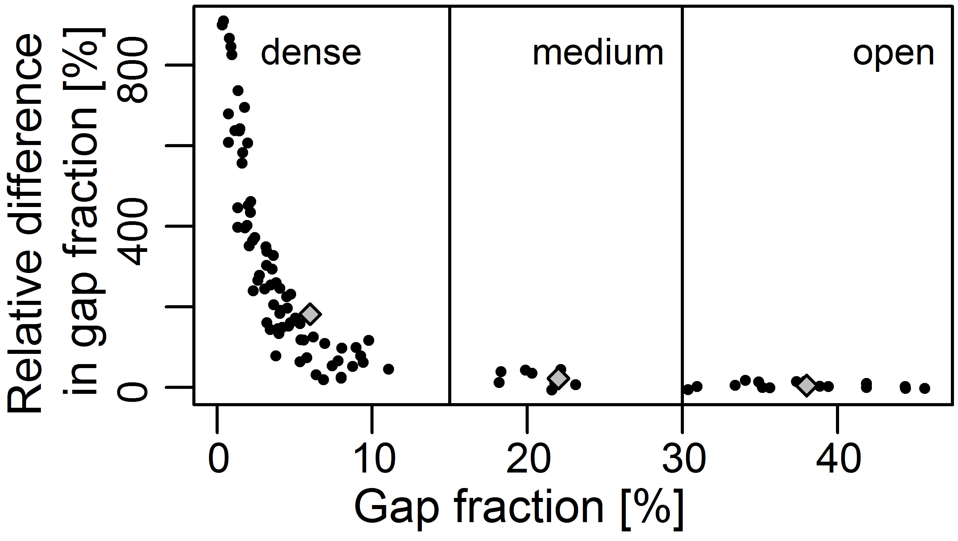
In all three strata, medians of gap fraction (Tab. 2) differed significantly between the two exposure methods (“open”: p<0.05; “medium”: p<0.05; “dense”: p<0.001). It was observed that differences in gap fraction were increasing on denser canopy locations. Relative differences sharply increased when gap fraction dropped below 15% (mean difference of 181.96%) and reached up to over 900% under very low gap fraction conditions (Fig. 5, Tab. 2).
Fig. 5 - Relative difference of gap fraction estimates derived from auto-exposed and non-overexposed photographs. Grey diamonds: mean difference per stratum.
Largest gap index (LGI) and number of gaps
In non-overexposed photographs, the mean LGI was 5.95% while in auto-exposed photographs it was 7.79% (Tab. 3); LGI medians differed significantly (p<0.001).
Tab. 3 - Mean (standard deviation in parenthesis) and median of Largest Gap Index (LGI) estimates.
| Stratum | non-overexposed | auto-exposed | ||
|---|---|---|---|---|
| Mean | Median | Mean | Median | |
| all | 5.95 (10.06) |
1.41 | 7.72 (10.06) |
3.52 |
| open | 24.54 (11.04) |
25.71 | 25.68 (11.17) |
27.22 |
| medium | 10.54 (6.70) |
9.30 | 13.99 (7.08) |
15.68 |
| dense | 1.37 (1.78) |
0.62 | 3.10 (2.53) |
2.19 |
In stratum “open”, medians did not differ significantly between auto-exposed and non-overexposed photographs (p=0.16), but significant differences were observed for medians in the strata “medium” (p <0.05) and “dense” (p<0.001). While the total difference between mean values was largest in stratum “medium”, relative differences were larger in stratum “dense”. Here, the LGI of auto-exposed photographs was on average 226% larger than the LGI of non-overexposed photographs.
In all strata, auto-exposed photographs tended to have higher mean numbers of gaps (Tab. 4). Differences of medians were highly significant in stratum “open” (p<0.001) and “dense” (p<0.001). Also medians calculated over all strata were significantly different between non-overexposed and auto-exposed photographs (p<0.001). In stratum “medium” the medians of number of gaps did not show significant differences (p=0.74).
Tab. 4 - Mean and median number of gaps within non-overexposed and auto-exposed photographs. Mean and median number of gaps <2000 pixel (<0.1% gap fraction) are in round parenthesis and gap fraction represented by gaps <2000 pixel are in square brackets.
| Stratum | non-overexposed | auto-exposed | ||
|---|---|---|---|---|
| Mean | Median | Mean | Median | |
| all | 2735 (2729) [2.31%] |
2682 (2678) [1.90%] |
3994 (3982) [4.58%] |
3778 (3767) [4.38%] |
| open | 1975 (1958) [2.91%] |
1680 (1658) [2.54%] |
2435 (2417) [3.19%] |
2322 (2292) [2.91%] |
| medium | 3283 (3268) [4.33%] |
3212 (3208) [3.94%] |
3487 (3740) [4.59%] |
2438 (2425) [4.04%] |
| dense | 2842 (2838) [1.95%] |
2794 (2793) [1.66%] |
4392 (4381) [4.89%] |
4627 (4614) [4.85%] |
Over all strata, 99.52% of differences in mean number of gaps could be allocated to changes in the number of small gaps with a size <2.000 pixel (or <0.1% gap fraction). In Tab. 4, 36.31% of the difference in mean gap fraction between exposure methods could be allocated to the difference in numbers of these small gaps. Still, the enlargement of large canopy openings due to overexposure accounted for the bigger share of 63.96%.
Discussion and conclusions
Our study made very clear that auto-exposed hemispherical photographs cannot be reliably interpreted. Other studies support these findings ([8], [80]): Zhang et al. ([80]) have shown that auto-exposed photographs overestimate gap fraction by 18-72% for medium and high density canopies and by 4-28% for open canopies. Our findings differed from these values and showed lower gap fraction overestimation under open canopies (on average 4.64%) and higher overestimation under dense canopies (on average 181.96%). These differences may be caused by different exposure metering and thresholding techniques applied by Zhang et al. ([80]). These authors used center-weighted exposure metering for auto-exposed photographs. Hence, exposure is influenced by the scene’s central feature, that is, if a gap is located at the center of a chosen scene exposure would be lower than if the center is covered by vegetation. In our study, luminance was assessed over a whole scene by matrix metering. Zhang et al. ([80]) used a manual thresholding technique for the binarization of photographs. This operator-dependent technique has been identified as a potential source of error in the processing of hemispherical photographs ([16], [31]). In our study, we replaced this technique with an automated thresholding technique which produced consistent and reproducible figures.
In forests, errors arising from auto-exposure occurred due to overexposure of vegetation. Compared to non-overexposed photographs, auto-exposed photographs contained more and larger gaps, and therefore, tended to overestimate gap fraction. By visual examination of auto-exposed photographs, it was observed that vegetation bordering canopy gaps was more illuminated than vegetation farther away from gaps. Larger gaps also tended to embrace fine structures, for example, in-growing branches and leaves that were brightly illuminated. In auto-exposed photographs most of these bright components were overexposed and appeared as solid white areas (Fig. 6), and consequently were mixed up with sky. The higher numbers of gaps appearing in auto-exposed photographs were due to the small size of gaps which permitted only very tiny fractions of light to enter, too small perhaps to be detected in non-overexposed photographs.
Fig. 6 - Subsets of hemispherical photographs taken at the same location. (A) Auto-exposed photograph: the vegetation at the border of gaps and branches and leaves growing into gaps were overexposed and disappeared. (B) Non-overexposed photograph (underexposed by -3.5 EVs): all relevant information was retained.
Auto-exposure resulted in increasing overestimation of gap fraction for decreasing canopy openness. Hence, relative distances in gap fraction among sample locations were not preserved by auto-exposure. Our study has also shown that underexposure with a fixed EV value, as done by, e.g., Jarcuska et al. ([29]) and Kato & Komiyama ([32]), is not suitable to standardize exposure of hemispherical photographs. The underexposure with a fixed EV value is just a modification of auto-exposure and does not avoid overexposure under dense canopy conditions. Gap fraction and lighting situation above the canopy affected the correct exposure and required variable values of underexposure ranging from -2 to -5 EVs in our study.
The wide availability of DSLR cameras with histogram display modes solves the problem of standardizing exposure for hemispherical photographs. In the reviewed literature we found only two other publications that describe a method similar to the Histogram Methods: Leblanc et al. ([36]) took three photographs (auto-exposed, underexposed by -1, and underexposed by -2 EVs) at each location. From these photographs, those were selected for analysis in which saturated pixels were limited to areas without vegetation. Macfarlane ([38]) adopted this approach but reduced subjectivity in the choice of exposure by selecting the darkest exposure having the maximum frequency of sky pixel luminance greater than 200. Nevertheless, Leblanc et al. ([36]) and Macfarlane ([38]) restricted themselves to a maximum underexposure of -2 EVs which was not enough to prevent overexposure under dense canopy conditions in our study. In addition, their methods require a subjective evaluation by the user to assess whether overexposure affects only parts of the sky or also parts of the canopy. In this respect, we directly experienced that it can be very difficult to judge whether overexposure is limited to sky pixels under dense canopy conditions. Therefore, we recommend to circumvent this subjective decision by a complete avoidance of overexposure as done by the Histogram Methods.
Due to problems related to auto-exposure, we strongly advise to apply either the method described by Wagner ([74]) or the Histogram Methods to determine exposure in hemispherical photography. These methods are independent of what camera and metering is used to assess the luminance of a scene (spot, center weighted, or matrix metering) which was identified as an error source in hemispherical photography ([8], [74]). Compared to the method described by Wagner ([74]), Histogram Methods have no need for reference measurements taken outside the forest stand. In this context, Yamamoto et al. ([79]) noticed that exposure is significantly impacted by changes in light conditions occurring in the time span between taking the reference measurement in the open land and the photograph in the forest. Zhang et al. ([80]) observed a difference of 1 EV within one hour between reference readings taken before and after entering the forest. This source of variation is eliminated by the Histogram Methods proposed here.
Acknowledgements
Our thanks are due to the Advisory Group on International Agricultural Research (BEAF) at the German Agency for International Cooperation (GIZ) and the German Ministry for Economic Cooperation (BMZ) for funding the research project MMC (“Making the Mekong Connected”, Project No. 08.7860.3-001.00) within which this study had been carried out. We are also grateful to all members of the MMC-project for their support. Especially, we thank Rhett D. Harrison for facilitating the data collection in Xishuangbanna Tropical Botanical Garden (XTBG). In addition, this study was supported by the CGIAR Research Program 6 on Forests, Trees and Agroforestry.
References
Gscholar
Gscholar
Gscholar
CrossRef | Gscholar
Online | Gscholar
Gscholar
Gscholar
Gscholar
Gscholar
Gscholar
Gscholar
Gscholar
Gscholar
Gscholar
Gscholar
Gscholar
Gscholar
Gscholar
Gscholar
Gscholar
Gscholar
Gscholar
Gscholar
Gscholar
Gscholar
Gscholar
CrossRef | Gscholar
Authors’ Info
Authors’ Affiliation
D Seidel
C Kleinn
Chair of Forest Inventory and Remote Sensing, Georg-August-Universität Göttingen, Büsgenweg 5, D-37077 Göttingen (Germany)
World Agroforestry Center, ICRAF-Kunming Office, Kunming, Yunnan 650201 (China)
Corresponding author
Paper Info
Citation
Beckschäfer P, Seidel D, Kleinn C, Xu J (2013). On the exposure of hemispherical photographs in forests. iForest 6: 228-237. - doi: 10.3832/ifor0957-006
Academic Editor
Francesco Ripullone
Paper history
Received: Jan 28, 2013
Accepted: Mar 26, 2013
First online: Jun 13, 2013
Publication Date: Aug 01, 2013
Publication Time: 2.63 months
Copyright Information
© SISEF - The Italian Society of Silviculture and Forest Ecology 2013
Open Access
This article is distributed under the terms of the Creative Commons Attribution-Non Commercial 4.0 International (https://creativecommons.org/licenses/by-nc/4.0/), which permits unrestricted use, distribution, and reproduction in any medium, provided you give appropriate credit to the original author(s) and the source, provide a link to the Creative Commons license, and indicate if changes were made.

Web Metrics
Breakdown by View Type
Article Usage
Total Article Views: 53852
(from publication date up to now)
Breakdown by View Type
HTML Page Views: 43887
Abstract Page Views: 3218
PDF Downloads: 5187
Citation/Reference Downloads: 67
XML Downloads: 1493
Web Metrics
Days since publication: 3964
Overall contacts: 53852
Avg. contacts per week: 95.10
Article Citations
Article citations are based on data periodically collected from the Clarivate Web of Science web site
(last update: Feb 2023)
Total number of cites (since 2013): 68
Average cites per year: 6.18
Publication Metrics
by Dimensions ©
Articles citing this article
List of the papers citing this article based on CrossRef Cited-by.
Related Contents
iForest Similar Articles
Research Articles
The estimation of canopy attributes from digital cover photography by two different image analysis methods
vol. 7, pp. 255-259 (online: 26 March 2014)
Short Communications
Estimation of canopy attributes of wild cacao trees using digital cover photography and machine learning algorithms
vol. 14, pp. 517-521 (online: 17 November 2021)
Technical Advances
Thermal canopy photography in forestry - an alternative to optical cover photography
vol. 8, pp. 1-5 (online: 07 May 2014)
Review Papers
Digital hemispherical photography for estimating forest canopy properties: current controversies and opportunities
vol. 5, pp. 290-295 (online: 17 December 2012)
Research Articles
Distribution of juveniles of tree species along a canopy closure gradient in a tropical cloud forest of the Venezuelan Andes
vol. 9, pp. 363-369 (online: 08 December 2015)
Research Articles
Quantifying the vertical microclimate profile within a tropical seasonal rainforest, based on both ground- and canopy-referenced approaches
vol. 15, pp. 24-32 (online: 27 January 2022)
Research Articles
Canopy temperature variability in a tropical rainforest, subtropical evergreen forest, and savanna forest in Southwest China
vol. 10, pp. 611-617 (online: 17 May 2017)
Research Articles
Is methane released from the forest canopy?
vol. 4, pp. 200-204 (online: 03 November 2011)
Research Articles
Analysis of canopy temperature depression between tropical rainforest and rubber plantation in Southwest China
vol. 12, pp. 518-526 (online: 09 December 2019)
Research Articles
Vertical position of dry mass and elemental concentrations in Pinus sylvestris L. canopy under the different ash-nitrogen treatments
vol. 8, pp. 838-845 (online: 25 March 2015)
iForest Database Search
Search By Author
Search By Keyword
Google Scholar Search
Citing Articles
Search By Author
Search By Keywords
PubMed Search
Search By Author
Search By Keyword


