
Single-tree influence on understorey vegetation in five Chinese subtropical forests
iForest - Biogeosciences and Forestry, Volume 5, Issue 4, Pages 179-187 (2012)
doi: https://doi.org/10.3832/ifor0623-005
Published: Aug 02, 2012 - Copyright © 2012 SISEF
Research Articles
Abstract
The aim of this study is to examine the effect of individual canopy tree on the species composition and abundance of understorey vegetation in subtropical forests, by applying a model for tree influence on understorey vegetation of boreal spruce forests developed by Økland et al. ([28]), according to the principles of Ecological Field Theory (EFT). The study was based upon five vegetation data sets, each with two subsets (vascular plants species and bryophytes species) from subtropical forests in south and southwest China. Optimal value of tree influence model parameters was found by maximizing the eigenvalue of a Constrained Ordination (CO) axis, obtained by use of the EFT-based tree influence index as the only constraining variable. One CO method, Redundancy Analysis (RDA), was applied to five vegetation data sets. The results showed that the optimal EFT tree influence models generally accounted for only a small part of the variation in species composition (the eigenvalues of RDA axes were low, amounted to 1-10% of total inertia). The higher eigenvalue-tototal-inertia ratio with RDA was interpreted as due mainly to the low species turnover along the tree influence gradient. Vascular plants and bryophytes species differed with respect to optimal parameters in the tree influence model, especially in a conifer dominated forest. Compositional turnover associated with tree influence indices was also generally low, although somewhat varies among study areas. Thus, it was concluded that single-tree EFT models may have limited suitability for studied subtropical forests; different optimal parameters in the tree influence model obtained for vascular plants and bryophytes species in two studied areas indicates that subtropical trees may impact vascular plants and bryophytes species in different ways; and trees may influence the understorey species composition more in a collective manner than through the influence of single individuals in studied subtropical forests.
Keywords
Competition, Understorey Vegetation, Bryophytes, Vascular Plants, Ecological Field Theory, Individual Tree Models
Introduction
Canopy trees may influence understorey species composition in an individual or collective manner ([26], [15], [28], [3], [22], [2], [6], [39]). In boreal forests, the properties of tree layer have proven important as determinants of understorey properties such as micro-climate, soil moisture, litter depth, litter distribution and light conditions ([30]). The distance from a given point on the forest floor to the nearest trees and the properties of these trees were important predictors of understorey species composition in boreal spruce forests ([28]). In tropical forests, properties of individual trees have proven to affect the distribution of lianas ([23]), but it remains unknown whether understorey species composition is more effectively predicted by local tree neighborhood or by average stand properties ([3], [45], [2]).
Ecological Field Theory (EFT) is a methodology for studying the interaction between plants of different size ([49], [17]). One of the main features of EFT is that it addresses interactions within a spatial context by determining a domain or size of the influence field. EFT models of tree influence express the effect of tree(s) on a given point x in the space as an exponential function of individual tree properties and the point’s distance to neighboring trees. EFT models have been applied to studies of single-tree influence on soil chemical properties, radiation at forest-floor level, seedling growth and understorey vegetation composition ([33], [28]) in boreal forests with one dominant tree species (e.g., Norway spruce, Scots pine). To our knowledge, however, EFT models have not yet been applied to assess the influence of single-tree properties on the composition of the understorey in (sub-) tropical forest ([47]).
Constrained Ordination (CO) is a family of multivariate statistical methods that optimize the fit of abundance data for species in sample plots to one or a set of explanatory (constraining) variable(s), under the assumption that variation in species abundance along the constraining variable(s) gradients is in accordance with a given species response model ([43]). The fit of data to an explanatory variable (provided the response model is appropriate) is measured by the eigenvalue of the CO axis ([41], [42], [4]). Eigenvalues corresponding to different constraining variables, measured in the same set of sample plots, may thus be compared ([35], [27], [1], [25]). Furthermore, constrained ordination is likely to be suited for finding the combination of single-tree influence index parameters that optimizes the fit to species abundance data ([28]).
Every CO method is derived from an ordination method by addition of a multiple regression step that makes the CO axes linear combinations of explanatory variables, while ordination axes are gradients in species composition per se, not influenced by measured explanatory variables ([41], [30]). The success of ordination methods in extracting the true gradient structure in a data set is, above all, dependent on the appropriateness of the species response model ([24]). In data sets with low β-diversity (low compositional turnover), species respond more or less linearly to the main gradients, while more species tend to have unimodal species responses in data sets with higher β-diversity ([24]). Thus, ordination methods based upon a unimodal species response model perform relatively better compared to methods based upon a linear model when β-diversity becomes higher ([24], [44]). Økland et al. ([28]) has tested the influence of response model appropriateness on the reliability of estimates of the variation explained by two CO methods, Redundancy Analysis (RDA) and Canonical Correspondence Analysis (CCA), concluding that the linear species response model in RDA was more appropriate than the unimodal species response model of CCA in single tree influence on understorey vegetation in a Norwegian boreal spruce forest.
For forests ranging from boreal via temperate ([32]) and subtropical ([5], [9], [52], [20]) to tropical ([46], [40]), gradients in understorey species composition were shown to be related to forest litter layer depth, topography, soil moisture, soil pH and soil nutrients, all of which co-vary along a gradient of overstorey tree density ([21], [18]). However, studies in five Chinese subtropical mixed conifer and broadleaf forests ([20]) revealed a distinct relationship between understorey species composition and forest density in only two out of five sites. This might suggest that the nature of the relationship between trees and understorey species composition may vary among different forest types, or that understorey species composition may be only weakly related to properties of the neighboring overstorey trees.
The aims of this study are: (1) to develop EFT models for single-tree influence on understorey vegetation for five mixed conifer and broadleaf subtropical forests; (2) to compare EFT model parameters obtained separately for vascular plants and bryophyte species; and (3) to discuss the importance of single-tree influence for understorey species composition and its possible influence mechanism in subtropical forests.
Materials and Methods
Study areas
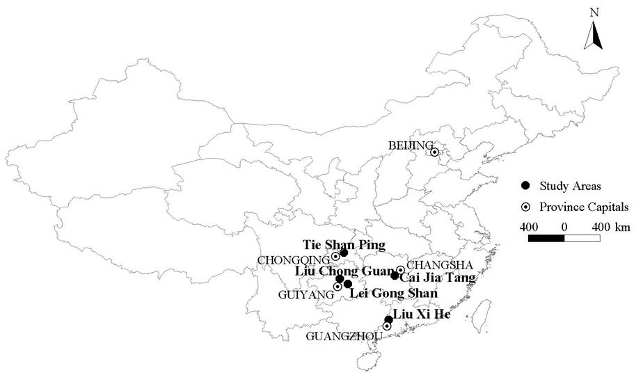
The five study areas were located in subtropical forests in south and southwest China (Tie Shan Ping, TSP; Liu Chong Guan, LCG; Lei Gong Shan, LGS; Cai Jia Tang, CJT; Liu Xi He, LXH - see Fig. 1). The climate in all five study areas is monsoonal, with dry winters and wet summers. Mean annual temperature and precipitation at the meteorological stations nearest to the study areas ranged between 15.3-22.0 °C and 1105-1736 mm, respectively (1971-2002, data from Chinese Meteorological Administration).
Fig. 1 - Map of China showing the position of the five study areas.
In all study areas parent material is sedimentary rocks such as sandstone and shale, except LXH which was dominated by granites. Soils belong to Haplic Alisol and Acrisol according to the Food and Agriculture Organization of the United Nations (FAO) classification system ([20]).
The study sites had a mixed conifer-broadleaf trees composition. Dominant species in TSP and LCG were Masson pine (Pinus massoniana L.) and Chinese fir (Cunninghamia lanceolata L.); in LGS Armand pine (Pinus armandii F.) and Chinese fir; in CJT Masson pine and sweet gum (Liquidambar formosana H.); and in LXH short-flowered machilus (Machilus breviflora B.) and itea (Itea chinensis H.&A. - Tab. 1). Tree stands in all five study sites were about 40-45 years old. Many of the forests were planted in the 1960s, after most Chinese forests were logged during the “Great Leap Forward” (1958-1962). At the time this study was carried out, four (TSP, LCG, LGS, and LXH) of the five study areas were protected by law. Three areas (TSP, LCG and LXH) have been exposed to pressure by tourism in recent years. However, there is no evidence of large-scale, human-induced, recent disturbances (except for the impact by “acid rain”) in any study area ([20]).
Tab. 1 - Summary characters of the study sites: number of trees (total and for two functional types) and number of tree species.
| Study area | Number of trees (absolute count) | Number of tree species |
||
|---|---|---|---|---|
| All trees |
Conifer trees | Broadleaf trees | ||
| Tie Shan Ping (TSP) | 167 | 116 | 51 | 23 |
| Liu Chong Guan (LCG) | 118 | 75 | 43 | 23 |
| Lei Gong Shan (LGS) | 151 | 120 | 31 | 26 |
| Cai Jia Tang (CJT) | 123 | 19 | 104 | 35 |
| Liu Xi He (LXH) | 184 | 1 | 183 | 50 |
Sampling, recording of trees and understorey vegetation
The five study areas (two south-facing, two north-facing, one east-facing), covering 4 200-10 800 m2 in Chinese subtropical forests, were selected so as to: (1) span across some of the regional climatic and geographical variation in Chinese subtropical forests; and (2) include most of the variation in the main local environmental gradients (e.g., soil nutrient content, soil moisture, tree density, etc.). The long axis of each study forest ran in the direction of maximum slope.
All the five study areas were irregular, 60 to 90 m broad and 70-120 m long. Characteristics of the stands, the details of approach and selection of study areas, placement of plots within each study area were given by Liu et al. ([20]).
In each of the five study areas we applied a stratified random sampling design: ten macro plots, each 10 × 10 m in size, were established in order to capture the higher possible variation along important ecological gradients (e.g., aspect, nutrient conditions, light supply, topographic conditions, soil moisture, etc.). Five 1-m2 vegetation plots were placed at random in each 10 × 10 m macro plot, resulting in 50 1-m2 plots in each study area. Each 1-m2 plot was divided into 16 subplots, 0.0625 m2 in size. All plots were permanently marked by subterranean aluminum tubes as well as with visible plastic sticks.
Within each macro plot, in the five sample stands, all trees higher than 2 m (overall 743 trees, of which 331 were conifer, 432 broadleaf - see Tab. 1) were mapped with respect to stem center and crown perimeter. Tree height (h) and diameter at breast height (dbh) were measured. The crown radius (k) was calculated as the mean of crown radii measured in eight cardinal directions.
Presence/absence of all understorey vascular plants and bryophyte species was recorded in each of the 16 0.0625-m2 subplots. Frequency (count of individuals at the subplot) was used as a measure of species abundance ([29]).
Single-tree influence model
We computed single-tree influence model used by Økland et al. ([28]). The model was developed based upon the principles of EFT ([49]) and six assumptions ([17], [16]):
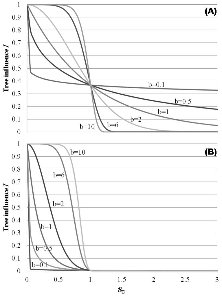
(1) The influence of tree i, Ii, at a particular point in space depend on: (i) the size of tree i relative to that of the largest tree encountered in the area (a parameter a specifies the exponent given to large vs. small trees - see eqn. 4, Fig. 2); and (ii) the distance from the point on the forest floor to the stem center of tree i (a parameter b specifies the exponent given to position close to the stem center relative to positions far away from the stem center - see eqn. 5, Fig. 3; another parameter c specifies the limit for tree influence, measured in crown radius units - see eqn. 6, Fig. 3). The influence of tree i is considered to be symmetrically distributed around the stem center.
Fig. 2 - The meaning of the parameter a in the EFT tree influence model (eqn. 10), explained by the tree influence factors φ (eqn. 4). Axis 1: parameter a, axis 2: factor φ. Parameter a determines the relative weight to be given to trees of different sizes; with a = 0, tree size has no effect on φ, while with a = 1 the relative importance of trees is proportional to their diameter at breast height. With 0 < a < 1, the weight varies within these limits.
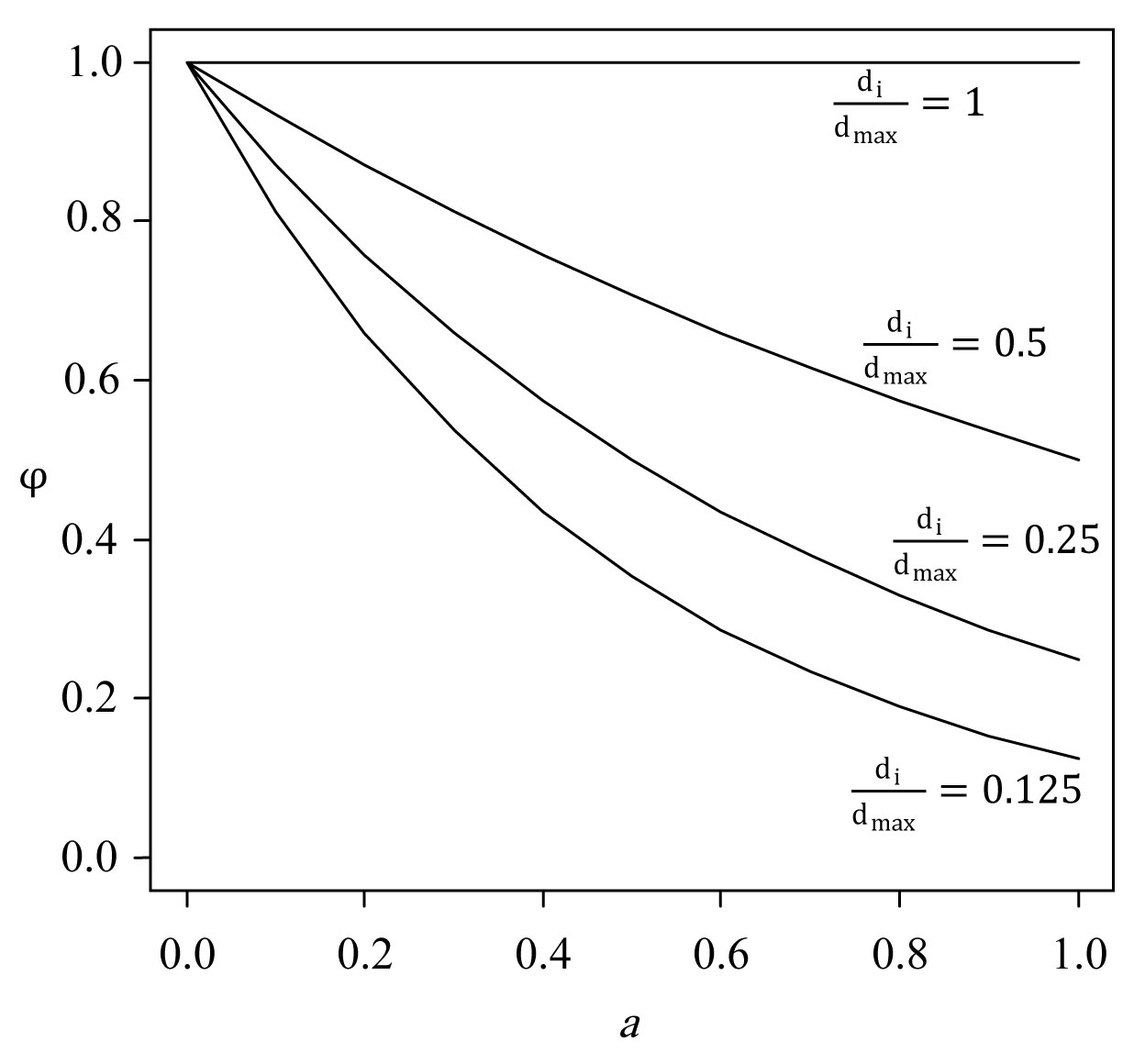
Fig. 3 - Meaning of parameters b and c in the EFT tree influence model (eqn. 10), explained by the tree influence I. Horizontal axis: factor SD (= s/ck); vertical axis 2: tree influence I. For simplicity, di = dmax. The parameter b can be visualized by replacing the parameter 5.298 with unity (5.298 => 1) in the tree influence model (eqn. 10): for b = 1, the tree influence with increasing dimensionless distance SD = s/ck from the tree is an exponential decay: e-. For b < 1 the tree influence decays faster than an exponential for SD < 1 and slower than an exponential for SD > 1. For b > 1 the tree influence starts off horizontally with little loss in influence (the derivative of the tree influence is zero at the stem, SD = 0) it decays slower than an exponential for SD < 1 and faster than an exponential for SD > 1, and b = 2 gives a Gaussian decay. This trend is shown for different values of b in (A). Note that for SD = 1 all curves have the same value e-1. By raising the functions in (A) to the power 5.298 all the curves that are less than unity everywhere are pushed down, and for SD = 1 all the curves have a value equal to (e-1)5.298 = e-5.298 = 0.005 as illustrated in (B). In the model SD = 1 or S = ck is defined as the maximal range of tree influence. Consequently, the interpretation of the parameter c is the maximal range of tree influence measured in units of crown radii k. For c = 4, the tree has no influence beyond four times crown radii.
(2) The influence of tree i on a point on the forest floor at distance s (measured in dm) from the stem center can be expressed as a product of two factors (eqn. 1):
where φi (hi; a) - the size factor - weighs trees by their size, e.g., by using the ratio of the height h of the i-th tree (measured in dm) to the highest tree encountered in the study area (which is arbitrarily given the value of φ = 1); ψi (si, k; b, c) - the distance factor - weighs points on forest floor in space by their distance s from the stem of the tree. The parameter ki denotes the crown radius of tree i (measured in dm). By arbitrarily defining ψ (0, ki; b, c) = 1 for a point situated at the stem center (s = 0), Ii takes on values between 0 and 1. The resulting model has three parameters, a, b and c (Fig. 2, Fig. 3), and expresses tree influence as a function of h, s and k.
(3) The size factor φi can be adequately modeled as a function of the height h of tree i and a parameter a´, which determines the exponent given to high vs. short trees (Fig. 2), as follows (eqn. 2):
where hmax is the height of the largest tree encountered in the study area. The height of a tree is allometrically related to the tree’s diameter d at breast height by the following equation (eqn. 3):
Because d is more easily measured than h, Økland et al. ([28]) used the following expression for the size factor φi (eqn. 4):
where a equals ra´ and dmax is the maximum diameter recorded for any tree in the study area.
(4) The distance factor ψi can be adequately modeled as a function of s and k based upon principles of EFT as follows (eqn. 5):
The parameter b in eqn. 5 determines the relative exponent given to positions close to the stem center relative to positions further away from the stem (Fig. 3). The parameter c´´ determines the zone of influence by tree i. The function ψi as given by eqn. 5 takes on positive values for all s, but in order to simplify the model, Økland et al. ([28]) truncated the its distribution by setting ψ = 0 for all s that corresponded to ψi values < 0.005. The value of s corresponding to ψ = 0.005, i.e., the limit for tree influence, was denoted by c´. The limit for tree influence measured in crown radius units, c (Fig. 3), was defined as (eqn. 6):
By inserting ψ = 0.005 and c·k for s in eqn. 5, Økland et al. ([28]) obtained the following expression for c´´ (eqn. 7):
Inserting eqn. 7 into eqn. 5 gave (eqn. 8):
(5) The crown radius k of a tree is allometrically related to the tree’s height h and, hence, to the diameter d of the tree. Økland et al. ([28]) therefore used the easily obtained information on d in their calculation of ψi, based upon the general relationship between k and d given by (eqn. 9):
Insertion of eqn. 9 in eqn. 8, and eqn. 8 and eqn. 4 in eqn. 1 gave the following expression for Ii (eqn. 10):
where t0 and t are constants.
(6) The total influence of all n trees adjacent to a point x, I(x), is adequately modeled by the multiplicative model (eqn. 11):
This model, with different values of a, b and c (Fig. 2, Fig. 3), was computed separately by using data on tree size and position relative to the plots in all study areas. Overall, 240 plots were used for vascular plant species, 50 in TSP, LCG, LGS and LXH, and 40 in CJT (excluding 10 plots located in pure bamboo stands). Overall, 212 plots were used for bryophytes species, 40 in TSP (excluding 10 plots devoid of bryophytes), 36 in LCG (excluding 14 plots devoid of bryophytes), 50 in LGS, 40 in CJT (excluding 10 plots located in pure bamboo stands) and 46 (excluding 4 plots devoid of bryophytes) in LXH, respectively.
Statistical analysis
Before determining the optimal values of the parameters a, b and c of the model, we used parameters k and d to estimate t0 and t by standard linear regression (eqn. 12):
For all combinations of the two vegetation groups in all five study areas, two species response models, CCA ([41], [42]) and RDA ([34], [41], [42]), were used to determine the values for parameters a, b and c in the EFT tree influence model (eqn. 10, eqn. 11) that maximized the eigenvalue of a constrained ordination axis constrained by the tree influence index ([28]). RDA assumes that species abundance values are linearly related to the explanatory variables, and CCA assumes unimodal distribution of species abundance values with respect to the explanatory variables. The two vegetation groups (all with 240 and 212 sample plots and subplot frequency data, respectively) used were: (1) vascular plants (330 species), and (2) bryophytes species (110 species).
The “vegan” package developed in R ([31]) was used for all multivariate analyzes. For each data set, species with a frequency lower than the median frequency were down-weighted by multiplication by the ratio of the species frequency and the median frequency ([8]). RDA was run after centering of species abundances, otherwise standard options were used.
Initial analyzes showed that the influence of parameters a versus parameters b and c on the variation explained by CCA axis, using modeled tree influence as the only constraining variable, was largely negligible (1-3%) and lower than the variation explained by RDA axis (1-10%), and all five vegetation data sets showed relative low β-diversity (low compositional turnover - Tab. 4). Therefore, as proved in the Norwegian boreal spruce forests ([28]), RDA was more appropriate than CCA in the study of single tree influence on understorey vegetation, hence, we only used RDA model in this study. Furthermore, as observed by Økland et al. ([28]) for boreal conifer forests, a = 0.6 turned out to be close to optimal for all data sets. We therefore used a = 0.6 in all our analyzes. Optimal values for parameters b and c for each of the 15 data sets (combinations of study area and species group) were found by running series of RDA analyzes, all with the tree influence index I as the only constraining variable, setting b = 0, 0.5, 1.0, 1.5, …, 10.0, and c = 1.0, 1.5, …, 10.0. In order to construct an overall model for all five sites, optimal values of parameters b and c obtained from each best-fitting models for the five study areas have been also compared.
Tab. 4 - Optimal models for tree influence. Variation is given in inertia units (IU), i.e., the eigenvalue of the RDA axis divided by total inertia (TI). Fr. of TI is the fraction of variation explained by a RDA axis standardized by dividing the eigenvalue of the axis by the total inertia. p values refer to a Monte Carlo test in which the variation explained by the best model was compared with those resulting from 9999 random permutations of the tree influence index based on this model (significance at level p < 0.01). Gradient length is the β-diversity (in S.D. units) associated with an rhCCA axis (see Methods) obtained by using the tree influence index as the only constraining variable.
| Study area |
Species group | Number of plots |
Parameter values | Variation explained | Length Fr. of TI |
p value | Gradient length |
|||
|---|---|---|---|---|---|---|---|---|---|---|
| b | c | Eigenvalue | TI | IU | ||||||
| TSP | All species | 50 | 0 | ≥1 | 1.925 | 61 | 0.032 | 0.043 | 0.004 | 1.363 |
| Vascular plants | 50 | 10 | 6.8 | 1.421 | 53 | 0.027 | 0.036 | 0.2145 | 2.348 | |
| Bryophyte species | 40 | 0 | ≥1 | 0.602 | 8 | 0.075 | 0.320 | 0.0055 | 0.653 | |
| LCG | All species | 50 | 5.9 | 4.9 | 5.407 | 61 | 0.089 | 0.023 | <0.0001 | 2.355 |
| Vascular plants | 50 | 5.8 | 4 | 2.35 | 44 | 0.053 | 0.028 | <0.0001 | 2.61 | |
| Bryophyte species | 36 | 5.8 | ≥5.8 | 3.11 | 17 | 0.183 | 0.098 | <0.0001 | 1.378 | |
| LGS | All species | 50 | 4.4 | 3 | 8.366 | 172 | 0.049 | 0.007 | <0.0001 | 2.407 |
| Vascular plants | 50 | 5.1 | 2.9 | 7.55 | 125 | 0.06 | 0.010 | 0.0001 | 2.301 | |
| Bryophyte species | 50 | 2.7 | 1 | 1.192 | 47 | 0.025 | 0.033 | 0.128 | 1.282 | |
| CJT | All species | 40 | 10 | 7.3 | 3.294 | 65 | 0.051 | 0.014 | 0.002 | 1.327 |
| Vascular plants | 40 | 9.7 | 9.8 | 2.412 | 49 | 0.049 | 0.026 | 0.0046 | 1.425 | |
| Bryophyte species | 40 | 10 | 6.1 | 0.890 | 16 | 0.056 | 0.172 | 0.0308 | 0.739 | |
| LXH | All species | 50 | 10 | 7.2 | 3.965 | 139 | 0.029 | 0.014 | 0.095 | 2.035 |
| Vascular plants | 50 | 10 | 7.2 | 3.735 | 117 | 0.032 | 0.007 | 0.0352 | 2.408 | |
| Bryophyte species | 46 | 1 | 1 | 0.559 | 22 | 0.025 | 0.066 | 0.3 | 1.393 | |
Regardless of the choice of model parameters, only trees closer than approx. 2.5 crown radius units from the mid-point of a sample plot were used for calculation of the index I, since the negligible influence played by trees farther away.
Given a set of parameter values, the variation explained by the tree influence index I was expressed as the eigenvalue of the first (and only) constrained ordination axis. Because total inertia (TI, the sum of all unconstrained eigenvalues of the corresponding PCA - Principal Components Analysis - or CA - Correspondence Analysis - ordination) is a univariate variable as a measure of the total variation in a vegetation data set ([25]), the “fraction of variation explained (Fr. of TI)” by a RDA axis was standardized by dividing the eigenvalue of the axis by the total inertia ([14], [4], [27]). After the optimal set of parameters had been found, a distribution-free Monte Carlo simulation test ([19]) was performed, in which the variation explained by the constraining variable was compared with the variation explained by each of 9999 randomized rearrangements (permutations) of this variable. The test statistics was the partial F-statistic, with model and residual sums of squares totaled across species ([44], [31]).
Differences in variation explained and compositional turnover (β-diversity, gradient lengths in S.D. units) between study areas and species groups were tested for significance using the Kruskal-Wallis test ([37] - α < 0.01). The strength of relationships between variation explained and gradient lengths was evaluated using the Kendall’s non-parametric correlation coefficient τ ([37]).
Results
The total number of conifer and broadleaf trees varied much among areas. The number of broadleaf trees was relatively high in LXH and CJT, and the opposite was true in TSP and LGS (Tab. 1). The diversity of tree species is relatively high in LXH, and relatively low in TSP and LCG (Tab. 1).
Tests of the regression model in eqn. 12 revealed strongly significant relationships between diameter at breast height (d) and crown radius (k). The regression parameters for the five study areas are presented in Tab. 2.
Tab. 2 - Relationship between tree measurements in all five study areas. All regressions were significant at p < 0.001. (Int 0): intercept; (t): regression coefficient (see eqn. 12).
| Study area |
Diameter at breast height (d, cm) |
Crown radius (k, dm) |
Parameter’s values |
Coefficient of determination |
n | ||
|---|---|---|---|---|---|---|---|
| Average | Standard deviation |
Average | Standard deviation |
||||
| TSP | 14.45 | 6.9 | 17.78 | 6.65 | t0 =6.062 t = 0.396 |
r2 = 0.309 | 167 |
| LCG | 18.09 | 9.87 | 20.01 | 7.67 | t0 =6.910 t = 0.360 |
r2 = 0.264 | 118 |
| LGS | 20.92 | 8.53 | 20.23 | 8.82 | t0 =3.428 t = 0.570 |
r2 = 0.363 | 152 |
| CJT | 11.3 | 6.59 | 14.15 | 6.85 | t0 =2.494 t = 0.705 |
r2 = 0.487 | 123 |
| LXH | 12.44 | 7.54 | 18.47 | 10.59 | t0 =2.270 t = 0.813 |
r2 = 0.517 | 184 |
The total number of vascular plant and bryophyte species recorded in both the plots and macro plots varied much among areas (Tab. 3). In the plots, the number of vascular plant species varied from only 44 in LCG to 125 in LGS, and the number of bryophyte species from only 8 in TSP to 47 species in LGS. In the macro plots, the ranking of areas remained the same as that obtained for the plot scale.
Tab. 3 - Number of species per plot and macro plot in each of the five study areas.
| Study area |
Species group | Number of species per plot |
Number of species per macro plot |
||
|---|---|---|---|---|---|
| Range | Median | Range | Median | ||
| TSP | Vascular plants | 2-12 | 6 | 13-23 | 19.5 |
| Bryophyte species | 1-6 | 3 | 1-9 | 5.5 | |
| LCG | Vascular plants | 1-10 | 5 | 7-20 | 13 |
| Bryophyte species | 1-8 | 3 | 0-12 | 6 | |
| LGS | Vascular plants | 7-25 | 13 | 20-32 | 24.5 |
| Bryophyte species | 1-12 | 7 | 6-17 | 12 | |
| CJT | Vascular plants | 2-10 | 6 | 15-28 | 21 |
| Bryophyte species | 1-7 | 4 | 0-4 | 1 | |
| LXH | Vascular plants | 3-23 | 11 | 23-50 | 34 |
| Bryophyte species | 1-7 | 3 | 2-18 | 5.5 | |
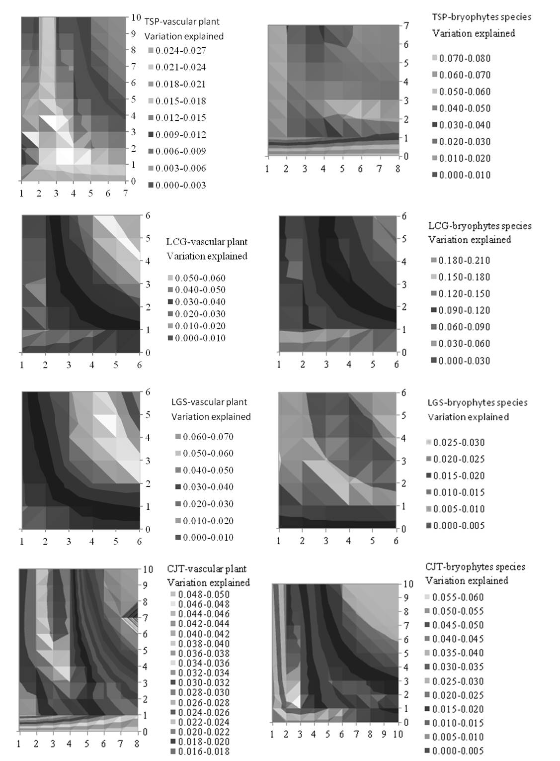
In each study area the variation in understorey species abundances accounted for the tree influence index varied systematically as a function of b and c. Near-optimal tree influence indexes (i.e., those accounting for the highest percent of the variation) were obtained over a wide range of b or c values for all 10 data sets (5 study sites × 2 vegetation groups - Fig. 4, Tab. 4). RDA ordination tri-plots of plots, species and optimal tree influence index (TI) are reported in Appendix 1.
Fig. 4 - Variation in species composition for the five study areas, each with two species groups, explained by the tree influence index, as a function of parameters b and c in eqn. 10 and eqn. 11. Variation explained is expressed as the ratio of the eigenvalue of the constrained ordination axis obtained by use of the tree influence index as the only constraining variable in an RDA constrained ordination, divided by the total inertia (see text for further explanation, see also Tab. 4). Axis 1 (horizontal, parameter c) and axis 2 (vertical, parameter b).
The maximum “fraction of variation explained” varied considerably among study areas and species groups (Tab. 4 - see also Appendix 1). The maximum explained variation was significantly higher than that associated to a random variable (p = 0.01) for nine out of 15 data sets (Tab. 4), without systematic differences among areas (Kruskal-Wallis test: χ2[4] = 6.47, p = 0.167, n = 15; 5 observations × 3 treatments) or species groups (Kruskal-Wallis test: χ2[2] =1.09, p = 0.581, n = 15; 3 observations × 5 treatments) or vascular plant species vs. bryophytes species (Kruskall-Wallis test: χ2[2] = 2.2, p = 0.532, n = 10; 2 observations × 5 treatments). The observed variance of vascular plants explained by tree influence was significantly larger than that expected by chance after Monte Carlo tests in LCG, LGS and CJT (Tab. 4, p <0.01). Analogously, the variance of bryophytes species accounted for tree influence was also significant after Monte Carlo tests in TSP and LCG (Tab. 4, p <0.01).
The optimal combination of the parameters b and c differed between study areas and species groups. Relatively high values for b (b=5.8 in LCG, b=5.1 in LGS) and low c (c=4.0 in LCG, c=2.9 in LGS) for vascular plant species were obtained in two (LCG, LGS) out of five areas (Tab. 4). In LCG, the models for vascular plants tend to have same value of b (b=5.8) and relative lower c (c=4.0) for vascular plant species than models for bryophyte species (b=5.8, c≥5.8).
In this investigation, study areas and species groups differed in the compositional turnover associated with tree influence best-fitting models, as estimated by rhCCA gradient lengths. Compositional turnover was invariably low for bryophyte species (0.65-1.4 S.D. units in the five areas), while it was > 2.3 S.D. units for vascular plants in TSP, LCG, LGS and LXH, and 1.3-1.5 S.D. units for vascular plants in CJT (Tab. 4). Compositional turnovers were not significantly different among areas (Kruskal-Wallis test: χ2[4] = 4.5, p = 0.343, n = 15), while significant differences were found among species groups (Kruskal-Wallis test: χ2[2] = 7.74, p = 0.021, n = 15).
Compositional turnover was not significantly related to the fraction of variation explained by optimal EFT models (Kendall’s τ = - 0.134, p = 0.486, n = 15).
Discussion
The five study areas in Chinese subtropical forests analyzed in this study showed strong differences with respect to properties of optimal EFT models for tree influence on the understorey vegetation, as demonstrated by the strong variation in parameters b and c. No unified EFT model could be constructed that was valid over the whole range of variation. Furthermore, parameters (0 ≤ b ≤ 10 and 1.0 ≤ c ≤ 10.0 - Tab. 4) of optimal models for Chinese subtropical forests strongly contrasted those obtained for boreal spruce forest understorey vegetation in Norway (b = 2.2 and c = 2.5) by Økland et al. ([28]). The above results indicate that forest ecosystems differing in dominant canopy trees and situated in different temperature zones are also likely to differ not only in the understorey species composition, but also in the strength and perhaps the mechanism by which the canopy influences the forest-floor environment. For instance, the gap structure in the tree layer (e.g., moving from full cover to openings between trees) has been found to be one of the 2-3 most important vegetation gradient in boreal forests ([30], [13]). Trees affect vascular plants and bryophytes in different ways: for bryophytes species, high tree influence was found within the crown perimeter, while vascular plants were influenced at larger distances from tree stems ([28]). However, in (sub-) tropical forests at least in our studied areas, tree-layer density, is found significantly related to vegetation gradient only in two out of five sites ([20]). The mechanism by which the understorey species composition is affected by the structure of the overstorey tree layer is complex ([20]) and remains uncertain ([3], [45], [2]).
In LCG, the difference between vascular plants and bryophytes with respect to parameter combinations that maximized variation explained by the tree influence index, may indicate that trees impact vascular plants and bryophytes in different ways. For instance, conifer dominated forests in acid rain polluted areas on soils poor in nutrients, vascular plants are limited primarily by low availability of water from the soil ([12]) and by high soil acidity ([20]). Trees influence soil moisture by canopy interception and, perhaps even more strongly, by root uptake of water which may occur over a considerable area ([48]). Higher soil moisture in gaps than below trees ([26], [30]) indicate that soil moisture is correlated with tree influence and tree stand density at both fine and broader scales. Furthermore, trees may influence in a similar way both soil acidity and moisture, since the acidification process directly depends on acid rain pollution ([20]). Indeed, the ordination analysis showed that sites with higher soil pH also tend to have higher vascular plant species number ([20]).
Tree influence on vascular plant species composition over distances extending 2.9-4.0 crown radius units away from the stem (c=4.0 in LCG and c=2.9 in LGS - Tab. 4) interacts with soil acidity and soil moisture as the most important determinants of vascular plant abundance. Soil texture and chemistry are additional co-varying factors likely to affect vascular plant composition along the gradient from below trees to openings between trees ([30]), as a consequence of the thick layer of loose litter normally occurring under crowns of large conifer trees.
Ordination results showed that bryophytes species are limited primarily by high litter layer depth in LCG ([20]). Higher litter layer depth below conifer trees than below broadleaf trees ([20]) indicates that litter layer depth is correlated with the types of canopy tree. In addition, PCA ordination of environmental variables in LCG showed that litter layer depth is correlated with the topography at both fine and broad scales. This may explain the tree influence on bryophytes species occurring over a certain distance from crown radius.
The mechanisms by which litter layer depth affects bryophytes may be linked to soil moisture and nutrients, since litter plays a major role in forest ecosystems, both as an inherent part of the nutrient and carbon cycling, and regulating microclimatic conditions on the ground ([36]). However, no significant relationships between litter layer depth and soil moisture/soil nutrients has been found in the studied area ([20]).
In LXH and for bryophytes species in CJT, both dominated by deciduous trees, variance of understorey species composition accounted for by tree influence did not differ from random expectation after Monte Carlo test (p>0.01 - Tab. 4). This may be due to the relatively dense tree coverage (personal field observation) and high forest species richness (Tab. 1) in subtropical broadleaf forests; a situation in which the understorey may be influenced by the overall structure of the forest canopy rather than to neighboring trees alone. Our results suggest that forests dominated by conifer trees (e.g., LCG, LGS) are fundamentally different from broadleaf forests with respect to the mechanism and the extent of tree influence on understorey vegetation, at least in studied subtropical areas.
However, if we consider the biological meaning of the parameters b and c of the optimal EFT models, the relationship between single trees and the understorey may be questioned. As previously mentioned, parameter b is an estimate of the relative distance off the stem at which tree influence reduces most rapidly (Fig. 3); for b < 1 tree influence rapidly decreases from the stem, while for very large b values (>> 1) the maximal reduction takes place further away from the stem (Fig. 3). Similarly, parameter c is an estimate for the distance off the stem (measured in crown radius units) at which tree influence decreases to 0.005 times the value at the stem center (see eqn. 7). For example, with c = 4, the maximum zone of influence of the largest observed tree (e.g., stem diameter = 54 cm (LXH), estimated crown radius = 5.35 m) is about 21.4 m (4 times the crown radius of approx. 5.35 m). Thus, from an ecological point of view, values for parameters b and c outside the range 1-6 hardly make sense (see Fig. 3). In our study the optimal value for b was > 6 for CJT and 0 for TSP, in which the variation in species abundances explained by the tree influence index was significant (Tab. 4).
This apparent paradox (significant variation in species composition tends to be explained by models whose parameters fall outside the meaningful range) may suggest that, in the studied subtropical forests, trees may influence the understorey vegetation in a collective manner rather than individually, e.g., through properties such as canopy cover ([38], [10]), throughfall light ([7], [11]), soil characteristics ([51]), etc. This hypothesis also agrees with our results of ordination analyzes of the understorey vegetation of the studied Chinese subtropical forests, where important explanatory factors are litter-layer depth, topography, soil pH and soil mineral nutrients ([20], [50]).
Conclusions and recommendations
Results from EFT models for tree influence on the understorey vegetation in Chinese subtropical forests may suggest that: (1) single-tree EFT models have limited suitability for subtropical forests; (2) different EFT model parameters, obtained for vascular plants and bryophytes species that maximized the variation explained by the tree influence index, indicates that subtropical trees may impact vascular plants and bryophytes species in the different ways; and (3) subtropical forests comprise many of ecosystem types, which differ with respect not only to variation in species composition along regional climatic and environmental gradients, but also with respect to the way the overstorey influences the understorey vegetation. Subtropical forests, at least those investigated in this study, generally have a closed canopy layer with multi-crown shapes and small canopy gaps, in which light, throughfall precipitation and canopy leaches may be redistributed on ground level in ways that are more or less unrelated to size and location of individual trees. However, this hypothesis should be further investigated. Furthermore, more research on gradient analyzes of forests ground vegetation and its relationships to environmental variables including tree influence index in a range of subtropical forests types are needed.
Acknowledgements
This study is part of a Sino-Norwegian joint effort for the Integrated Monitoring Program on Acidification of Chinese Terrestrial System (IMPACTS). The IMPACTS project was financially supported by the Norwegian government through NORAD (The Norwegian Agency for Development Co-operation) and Chinese government through MOE (Ministry of Environment). We acknowledge all those who supported the project. We are especially grateful to Quanru Liu, Tonje Økland and Harald Bratli who were involved in fieldwork.
References
Gscholar
Gscholar
Gscholar
Gscholar
Gscholar
Gscholar
Gscholar
Gscholar
Gscholar
Gscholar
Authors’ Info
Authors’ Affiliation
Centre for Ecology and Economics, Norwegian Institute for Air Research, P.O. Box 100, 2027 Kjeller (Norway)
Department of Research and Collections, Natural History Museum, University of Oslo, P.O. Box 1172, Blindern, 0318 Oslo (Norway)
Corresponding author
Paper Info
Citation
Liu H-Y, Halvorsen R (2012). Single-tree influence on understorey vegetation in five Chinese subtropical forests. iForest 5: 179-187. - doi: 10.3832/ifor0623-005
Academic Editor
Renzo Motta
Paper history
Received: Oct 24, 2011
Accepted: Jun 30, 2012
First online: Aug 02, 2012
Publication Date: Aug 29, 2012
Publication Time: 1.10 months
Copyright Information
© SISEF - The Italian Society of Silviculture and Forest Ecology 2012
Open Access
This article is distributed under the terms of the Creative Commons Attribution-Non Commercial 4.0 International (https://creativecommons.org/licenses/by-nc/4.0/), which permits unrestricted use, distribution, and reproduction in any medium, provided you give appropriate credit to the original author(s) and the source, provide a link to the Creative Commons license, and indicate if changes were made.

Web Metrics
Breakdown by View Type
Article Usage
Total Article Views: 47439
(from publication date up to now)
Breakdown by View Type
HTML Page Views: 39596
Abstract Page Views: 2330
PDF Downloads: 4434
Citation/Reference Downloads: 19
XML Downloads: 1060
Web Metrics
Days since publication: 4282
Overall contacts: 47439
Avg. contacts per week: 77.55
Article Citations
Article citations are based on data periodically collected from the Clarivate Web of Science web site
(last update: Feb 2023)
Total number of cites (since 2012): 2
Average cites per year: 0.17
Publication Metrics
by Dimensions ©
Articles citing this article
List of the papers citing this article based on CrossRef Cited-by.
Related Contents
iForest Similar Articles
Research Articles
Individual-based approach as a useful tool to disentangle the relative importance of tree age, size and inter-tree competition in dendroclimatic studies
vol. 8, pp. 187-194 (online: 21 August 2014)
Research Articles
Local ecological niche modelling to provide suitability maps for 27 forest tree species in edge conditions
vol. 13, pp. 230-237 (online: 19 June 2020)
Research Articles
Diameter growth prediction for individual Pinus occidentalis Sw. trees
vol. 6, pp. 209-216 (online: 27 May 2013)
Research Articles
Individual tree mortality of silver birch (Betula pendula Roth) in Estonia
vol. 9, pp. 643-651 (online: 04 April 2016)
Research Articles
Comparison of traits of non-colonized and colonized decaying logs by vascular plant species
vol. 11, pp. 11-16 (online: 09 January 2018)
Research Articles
Spatio-temporal modelling of forest monitoring data: modelling German tree defoliation data collected between 1989 and 2015 for trend estimation and survey grid examination using GAMMs
vol. 12, pp. 338-348 (online: 05 July 2019)
Research Articles
Local neighborhood competition following an extraordinary snow break event: implications for tree-individual growth
vol. 7, pp. 19-24 (online: 14 October 2013)
Research Articles
Vascular plants diversity in short rotation coppices: a reliable source of ecosystem services or farmland dead loss?
vol. 13, pp. 345-350 (online: 17 August 2020)
Research Articles
Quantifying forest net primary production: combining eddy flux, inventory and metabolic theory
vol. 10, pp. 475-482 (online: 12 April 2017)
Research Articles
Deriving tree growth models from stand models based on the self-thinning rule of Chinese fir plantations
vol. 15, pp. 1-7 (online: 13 January 2022)
iForest Database Search
Search By Author
Search By Keyword
Google Scholar Search
Citing Articles
Search By Author
Search By Keywords
PubMed Search
Search By Author
Search By Keyword


