Responses of European forest ecosystems to 21st century climate: assessing changes in interannual variability and fire intensity
iForest - Biogeosciences and Forestry, Volume 4, Issue 2, Pages 82-99 (2011)
doi: https://doi.org/10.3832/ifor0572-004
Published: Apr 05, 2011 - Copyright © 2011 SISEF
Research Articles
Collection/Special Issue: IUFRO RG 7.01 2010 - Antalya (Turkey)
Adaptation of Forest Ecosystems to Air Pollution and Climate Change
Guest Editors: Elena Paoletti, Yusuf Serengil
Abstract
Significant climatic changes are currently observed and, according to projections, will be strengthened over the 21st century throughout the world with the continuing increase of the atmospheric CO2 concentration. Climate will be generally warmer with notably changes in the seasonality and in the precipitation regime. These changes will have major impacts on the biodiversity and the functioning of natural ecosystems. The CARAIB dynamic vegetation model driven by the ARPEGE/Climate model under forcing from the A2 IPCC emission scenario is used to illustrate and analyse the potential impacts of climate change on forest productivity and distribution as well as fire intensity over Europe. The potential CO2 fertilizing effect is studied throughout transient runs of the vegetation model over the 1961-2100 period assuming constant and increasing atmospheric CO2 concentration. Without fertilisation effect, the net primary productivity (NPP) might increase in high latitudes and altitudes (by up to 40 % or even 60-100 %) while it might decrease in temperate (by up to 50 %) and in warmer regions, e.g., Mediterranean area (by up to 80 %). This strong decrease in NPP is associated with recurrent drought events occurring mostly in summer time. Under rising CO2 concentration, NPP increases all over Europe by as much as 25-75%, but it is not clear whether or not soils might sustain such an increase. The model indicates also that interannual NPP variability might strongly increase in the areas which will undergo recurrent water stress in the future. During the years exhibiting summer drought, the NPP might decrease to values much lower than present-day average NPP even when CO2 fertilization is included. Moreover, years with such events will happen much more frequently than today. Regions with more severe droughts might also be affected by an increase of wildfire frequency and intensity, which may have large impacts on vegetation density and distribution. For instance, in the Mediterranean basin, the area burned by wildfire can be expected to increase by a factor of 3-5 at the end of the 21st century compared to present.
Keywords
Productivity, Soil water, Fire disturbance, Climate change, Modelling
Introduction
Climate warming raises many questions about living organisms and ecosystems. Among these, there are considerable interest in species or biome distribution prediction, carbon cycling and impacts of droughts on ecosystems and forest fires.
The problem of species distribution is mainly related to biodiversity protection. According to Thuiller et al. ([86]), a growing literature is bringing convincing proofs that changes in regional climates have already pushed species to adapt their ranges, that some species are altering their phenology and that others are in danger of extinction, or have become extinct. At the present time, biodiversity loss is mainly due to habitat loss in quantity and quality, excess of harvest pressure and pollutants ([77]). Nevertheless, Thuiller et al. ([86]) point out recent calls to account for the climate change and the related dynamic nature of biodiversity in conservation management programs.
The challenge of carbon cycling studies is double. On the one hand, it is important to determine how each one of the ecosystems acts, as a source or as a sink of greenhouse gases to produce a global picture of carbon cycling and refine projections ([12], [73], [84]). In terrestrial ecosystems, climate change will affect primary production, respiration, soil carbon stocks and fire in contrasted ways. According to model projections ([62], [15], [73]), temperature rise could increase net primary production by several tens of percents in various ecosystems but only when coupled with effective fertilizing effect of CO2 and precipitation increase; otherwise, only negative changes were obtained. On the other hand, farm lands but also natural habitats and semi-natural areas such as managed forests and savannahs furnish various services and goods including the source of natural productions (timbers, firewood, medicinal matters, fodder, genetic resources, etc.) in addition to their ecological functions ([16]). Accurately quantifying their values would help to implement sustainable practices and to promote the conservation of the ecological function of carbon sink and eventually of the biodiversity. Here, models reveal contrasted responses to future climate, from positive to negative effects on the services and goods but mainly increased vulnerability ([78]).
Climate projections also indicate changes in climate variability and frequency of extreme events ([22], [37], [38], [75]). Since many biological processes undergo sudden shifts at particular thresholds for temperature or precipitation, altered meteorological variability has long-term consequences for ecosystem composition, functioning and carbon storage ([61]). Changes in the frequency of droughts or extreme seasonal precipitation might lead to physical and behavioural changes in a few species and to dramatic changes in the distributions of many other species ([72]). In European regions already submitted to fire disturbance, burned area would increase under most of the scenarios owing to increased summer drought frequency ([78]). Moreover, Flannigan et al. ([26]) are inclined to conclude to a general increase in burned area and fire occurrence even in the temperate and boreal regions and that this trend should continue in a warmer world. To improve projections, they particularly suggest to take into account the role of policy, practices and human behaviour because most of the global fire activity is directly attributable to people.
Process-based dynamic vegetation models are tools of choice to address to the study of the above problems. They can simulate the growth of various levels of primary producers, from species ([10], [49], [36], [41]), to “plant functional types” ([82]) or to “biological affinity groups of species” (BAGs - [51]) and eventually of different parts of the plants (roots, branches, stems, leaves, etc.) which could be useful to compute goods and their reactions to the changing environment. They could explicitly calculate the cycling of important environmental components like water or carbon ([31]). They could be upgraded with additional processes as far as needed (seed dispersal, insect disease, etc.).
In this paper, a new version of the CARAIB (Carbon Assimilation in the Biosphere) process-based dynamic vegetation model ([93] with changes made notably by [71] and [52]) is used to investigate the impacts of climate change on European forest ecosystems and to assess, most specifically, the changes in the interannual variability of soil water and primary productivity as well as fire intensity. Transient runs (1961-2100) with an improved module for plant spatial dynamics (plant competition and biogeography module), coupled to a fire module, are performed to follow the future evolutions of forest productivity and fires. In the new competition and biogeography modules, the description of species/BAG establishment, competition and mortality due to stresses and disturbances has been improved and these processes are now explicitly represented. The Bioclimatic Affinity Groups (BAGs), classification based on vegetation groups’ climatic tolerances and requirements, are for the first time used for future projections. Thus, the improved modules allow to map future changes in biome distribution and to identify areas where stresses on vegetation, especially water stress, might increase in the future. As terrestrial ecosystems may be affected by changes in variability almost as much as by changes in mean climate ([46], [61]), how future climate variability will affect ecosystem functioning could become a central question. Many studies, at the local ([39], [19], [61]), regional ([9], [2]) and global scales ([60]) looked into the responses of terrestrial ecosystems (carbon balance, etc.) to current climate variability but very few addressed the effects of future climate variability change. Here, at the European scale, we examine the consequences of future changes in climate interannual variability on soil water, drought episodes and their impacts on primary productivity taking also into account the potential role of CO2 fertilization. Moreover, in relation to water stress, the expected change in wildfire is analysed with the model.
Material and methods
CARAIB model
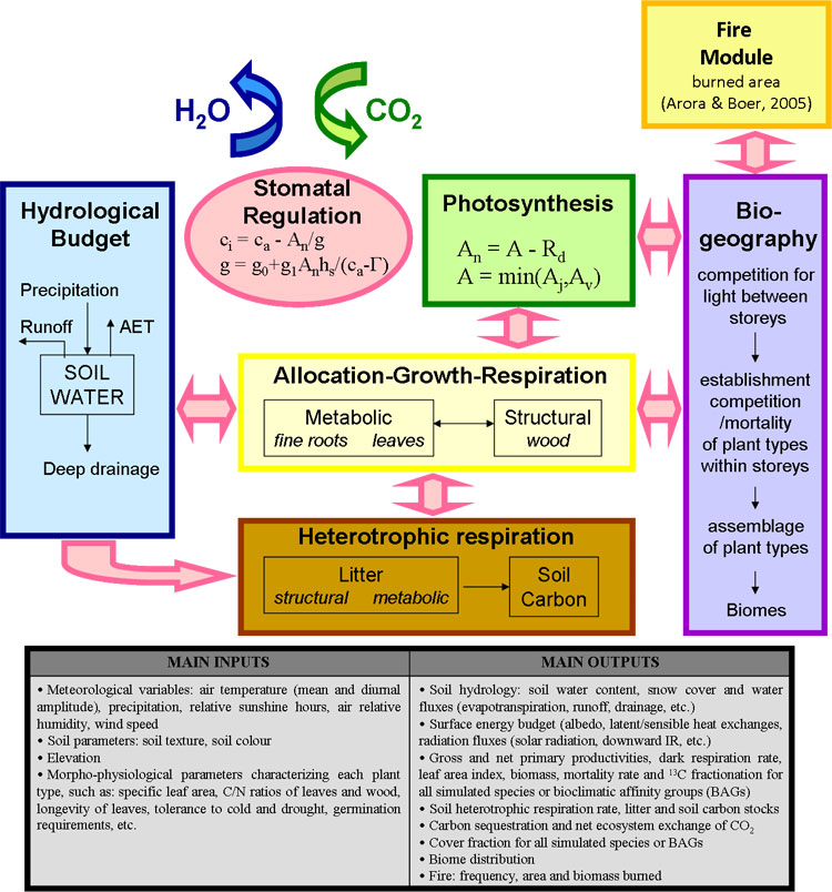
The CARAIB model ([92], [71], [52], François et al. submitted) is a large-scale vegetation model, originally designed to study the role of vegetation in the global carbon cycle at present ([93], [67], [31]) or in the past ([27], [28], [29], [30]). It is composed of several modules (Fig. 1) describing respectively: (1) the hydrological budget; (2) canopy photosynthesis and stomatal regulation; (3) carbon allocation and plant growth; (4) heterotrophic respiration and litter/soil carbon dynamics; (5) plant competition and biogeography; and (6) fire disturbance. In the present study, modules 2 and 5 have been improved and the fire module implemented.
Fig. 1 - Diagram illustrating the structure of the CARAIB model and summarizing its main input and output variables.
The hydrological module ([45], [29]) evaluates the average soil water content in the root zone, the snow cover and all related water fluxes.
The canopy photosynthesis and stomatal regulation module. Canopy photosynthesis is based on Farquhar et al.’s ([24]) model for C3 and Collatz et al. ([14]) for C4 plants. Stomatal conductance (gs) is related to the net assimilation using the parameterization developed by Ball et al. ([5]) - eqn. 1:
where g0 is the minimum conductance, g1 is a constant which can be dependent on plant type, An is the leaf net assimilation, RH is the relative humidity and ca is the CO2 concentration in the canopy air. Following Van Wijk et al. ([90]), in this relationship, g1 was multiplied by a soil water dependent factor fs (eqn. 2):
where S = (SW-WP)/(FC-WP) with SW the soil water content, WP the wilting point and FC the field capacity. The constants in this relationship are calibrated in such a way that fs becomes equal to 0 at the wilting point and tends to 1 at the field capacity. In our model, fs was slightly modified to introduce a dependence on the plant type, i.e., S was replaced by an effective soil water parameter, Seff (eqn. 3):
where Smin,spec is a species-dependent water threshold at which mortality occurs in the model (see below). The scaling of photosynthesis from leaves to canopy is now performed using the De Pury & Farquhar ([17]) scheme. Since this scheme already integrates radiative transfer within the canopy, the multiple layers computing for photosynthesis were suppressed and photosynthesis calculated once for each BAG taking into account the determined LAI. The incoming solar flux for the understorey is computed taking into account the absorption by the overstorey. This absorption results from the mean value due to each BAG present in the overstorey (cfr. plant competition and biogeography module).
The carbon allocation and plant growth module ([71]) allocates photosynthetic products to the metabolic (leaves and fine roots) and structural (wood and coarse roots) carbon reservoirs. This module also evaluates the autotrophic respiration and litter production fluxes.
The heterotrophic respiration and litter/ soil carbon module ([67]) calculates heterotrophic respiration rates, as well as the time evolution of metabolic litter, structural litter and soil carbon reservoirs.
The plant competition and biogeography module evaluates cover fraction of all Bioclimatic Affinity Groups (BAGs - [51]) on each pixel of the studied area. BAGs are defined as plant taxa gathered on the basis of vegetation morphology (height of the plant (tree/shrub/herb) and shape of leaves (needle/broad leaf)), phenology (deciduous/evergreen), and climatic affinity. To define these groups, geographical ranges of European plants were computed using discriminant analysis on monthly mean climatic data (monthly means of precipitation, wet-day frequency, mean and minimum temperatures, diurnal temperature range, percentage of sunshine hours and ground frost frequency - [68]) and growing degree days above 5 °C (GDD5).
The establishment of a BAG on a grid cell depends on the availability of free space on this grid cell and on the BAG climatic requirements for germination. The relevant variables controlling germination are the yearly sum of the daily temperatures above 5 °C (GDD5), the coldest monthly mean night temperature (Tcm) and the minimum monthly soil water content (SW). For germination to be possible in a given year, the values of these variables must be either lower (Tcm and SW) or higher (GDD5) than respective thresholds (Tmaxg, SWmaxg and GDD5ming) defined for each BAG (Tab. 1). All these thresholds are derived by calculating given percentiles in the observed BAG distributions (François et al. submitted). To avoid discontinuities, probability of germination is calculated through a truncated error function (erf) centred on the threshold with a fixed width corresponding to a standard deviation of 5% (GDD5 and SW) or 3 °C (Tcm).
Tab. 1 - BAG-dependent parameters controlling plant stress and germination. Soil water thresholds SWmins and SWmaxg refer to available soil water in relative units, i.e., in terms of the variable (W-WP)/(FC-WC) where W, WP and FC are respectively the soil water content, the wilting point and the field capacity in mm - see Laurent et al. ([51]) for a more detailed BAG list.
| N | BAG composition | Tmins (°C) |
Swmins | GDD5ming (°C day) |
Tmaxg (°C) | Swmaxg |
|---|---|---|---|---|---|---|
| 1 | Achillea, Alchemilla, Angelica, Campanula, etc. | -41.2 | 0.036 | 497 | 2.8 | - |
| 2 | Brassicaceae, Ranunculaceae, etc. | -40.7 | 0.098 | 519 | 2.6 | - |
| 3 | Anthemis, Artemisia, Bidens, Calystegia, etc. | -40.7 | 0.02 | 546 | 2.8 | - |
| 4 | Asteroideae, Cichorioideae, Poaceae, etc. | -50 | 0.02 | 50 | - | - |
| 5 | Anemone, Gypsophila, Helleborus, etc. | -41.6 | 0.042 | 443 | 2.9 | - |
| 6 | Ephedra, Ulex | -25.9 | 0.127 | 1642 | 2 | - |
| 7 | Alnus viridis, Arctostaphyllos alpinus, Betula nana, etc. | -40.4 | 0.289 | 529 | -2.2 | - |
| 8 | Frangula alnus, Lonicera, Prunus, Rubus, Sorbus, Vaccinium, Viburnum | -41.3 | 0.074 | 497 | 2.7 | - |
| 9 | Berberis vulgaris, Crataegus, Genista, Rhamnus, Sambucus, etc. | -29.2 | 0.085 | 1307 | 1.6 | - |
| 10 | Arctostaphyllos uva-ursi, Calluna vulgaris, Daphne | -41.3 | 0.093 | 558 | 2.7 | - |
| 11 | Buxus sempervirens, Hedera helix, Ilex aquifolium, Ligustrum vulgare, Viscum | -20.6 | 0.088 | 1458 | 2.2 | - |
| 12 | Cistus, Myrtus communis | -7.9 | 0.073 | 2677 | - | 0.383 |
| 13 | Betula, Salix | -40.7 | 0.101 | 523 | 2.5 | - |
| 14 | Alnus, Alnus glutinosa, Corylus avellana, Quercus, Quercus robur, Populus, etc. | -38.6 | 0.085 | 583 | 3.5 | - |
| 15 | Acer, Fraxinus, Fraxinus excelsior, Tilia cordata, Ulmus | -31.8 | 0.125 | 1153 | 1 | - |
| 16 | Acer campestre, Carpinus betulus, Fagus sylvatica, Tilia platyphyllos | -21.9 | 0.116 | 1602 | 1.4 | - |
| 17 | Castanea, Juglans, Ostrya, Quercus pubescens | -15.8 | 0.158 | 2006 | 1.5 | - |
| 18 | Olea europaea, Pistacia, Phillyrea, Quercus ilex, Quercus suber | -7.8 | 0.07 | 2695 | - | 0.466 |
| 19 | Larix decidua | -39.8 | 0.344 | 808 | -3.3 | - |
| 20 | Picea abies, Pinus, Pinus sylvestris | -41.5 | 0.095 | 555 | 2 | - |
| 21 | Abies | -38.8 | 0.29 | 1048 | -4.1 | - |
| 22 | Cupressaceae, Juniperus, Juniperus communis | -39.8 | 0.107 | 512 | 2.2 | - |
| 23 | Pinus cembra | -22.4 | 0.522 | 550 | -7.3 | - |
| 24 | Abies alba, Taxus baccata | -19.5 | 0.183 | 1472 | 0.1 | - |
| 25 | Cedrus, Pinus halepensis, Pinus pinaster | -8.3 | 0.084 | 2537 | - | 0.415 |
The initialisation of BAG cover fractions is performed assuming equal fractions for all germinated BAGs. An initial biomass of 5 g C m-2 for herb and shrub BAGs or 10 g C m-2 for tree BAGs. The cover fractions are estimated separately in each storey once a year after allocation of photosynthetic products to plant reservoirs. BAG fraction decreases are calculated daily and summed over the year. Mortality occurs owing to ageing mortality, thermal stress, water deficit stress and fire disturbances. Ageing death rate is inversely proportional to the rough estimates of BAG maximum life time, i.e., 5 yr for perennial herbs, 13 yr for shrubs and 100 yr for trees. These life times take into account mortality due to events, climatic (storms) or not (diseases), which are not simulated by CARAIB. Every year, corresponding fractions are removed from the BAG covers. Temperature and water stresses occur when 5-day running means of temperature and soil water content fall below prescribed thresholds (Tmins, SWmins) again determined for each BAG from its observed distribution (Tab. 1). Assuming a one month maximal survival time, 1/30 of the BAG fraction cover is removed daily in those conditions. To avoid numerical oscillations, the thermal stress begins 3°C above Tmins and is complete 3 °C below, while for water stress the limits are fixed to +5% and -5% of SWmins, also using an erf function as above. Finally, for fire disturbances (cfr. fire module), BAG mortality is proportional to area burned on the pixel. Mortality creates gaps in the vegetation cover. These are then filled with seeds of BAGs that can establish under current climatic conditions either BAGs that were already present on the grid cell or newly established BAGs (no dispersal rate limitations). Within the gap, the cover fraction of the established BAGs is assumed to be proportional to the BAG net primary productivity (NPP). This is the NPP of the previous year for the BAGs which were already present and 5 g C m-2 yr-1 (herbs and shrubs) or 10 g C m-2 yr-1 (trees) for newly established BAGs (consistently with the above initial biomass).
The fire module developed in CARAIB ([54]) is largely inspired by the approach implemented in the dynamic global vegetation CTEM model (Canadian Terrestrial Ecosystem Model - [4]). On a given grid cell, the emergence of a fire is conditioned by the three factors of the fire triangle: the availability of fuel (biomass, litter), the combustibility of the fuel (soil moisture) and the presence of a source of ignition (natural or anthropogenic). If one of these factors is missing, the fire cannot occur. The three constraints, considered in terms of probability, allow to calculate a probability of fire occurrence (Pf = Pb Pm Pi). Pb is the probability of fire conditioned on the available above-ground biomass (leaf, stem and litter pools averaged over all BAGs), Pm is the probability of fire conditioned on the soil moisture in the root zone and Pi is the fire occurrence probability linked to ignition source. The natural ignition constraint is represented by a “lightning scalar” linked to cloud-to-ground lightning frequency (flashes km-² month-1 - [4]). Here, the probability of fire ignition due to human causes is not taken into account consistently with the hypothesis of a potential natural vegetation reconstructed by the model. This choice of simulating natural fires with natural vegetation will prevent us from making a detailed comparison with actual fires. Moreover, this is the most parsimonious choice to simulate fires in the future. Indeed, despite the strong effect of humans on fires through ignition but also through management and land-cover change, human behaviour is extremely difficult to simulate ([26]) and remains a challenge for DVMs. Consequently, in our study, the aim is only to simulate the impacts of climate change on fires but not the impacts of the changes in the human factors since the latter would require the use of a dynamic land-use model. Once the probability of fire occurrence is established, the area burned on the grid cell can be calculated. It is taken elliptical in shape with point of ignition at one of the foci. The fire spread rate is a function of soil moisture and wind speed. Fire duration controls the maximum size of this ellipse that will be reached. It depends on an extinguishing probability parameter set to a fixed value as a first approximation. Again the extinguishing probability may depend on the human behaviour through land-use and fighting efforts. Since the future evolution of these factors is almost impossible to assess, it is another reason to restrict the analysis to natural systems.
Biome assignment scheme. CARAIB produces as outputs the cover fraction of all BAGs on each grid cell of the studied region. However, it is useful to transform this information on the abundance of plant types into a biome type characterizing each grid cell. Such a biome assignment scheme is useful essentially for visualizing the model results, but should not be used for comparing these results with the data. Indeed, the biome limits are rather imprecise and the biome classification generally varies from one author to the other. This biome assignment scheme is presented in Tab. 2. It will be used to provide synthetic maps illustrating the overall vegetation distribution in the model. The scheme contains a set of threshold conditions on GDD5, total NPP (NPPtot) and LAI of the grid cell (LAItot), the ratio of herbaceous NPP to tree NPP (R), the LAI of trees (LAItree) and the fraction of different types of trees. Most important thresholds are: permanent ice or polar desert is assumed to occur for GDD5 < 50, (extreme) desert for NPPtot < 0, tundra for 50 ≤ GDD5 ≤ 700 and LAItree < 0.8, semi-desert for NPPtot > 10 and LAItot < 0.3; grasslands occur for R > 0.4 and LAItree < 0.3, open woodlands for R > 0.4 and LAItree <0.3; forests occur for R > 0.4, their types being determined by the relative abundances of the different tree BAGs present in the over-storey.
Tab. 2 - Biome assignment scheme used in CARAIB. (GDD5): growing-degree-days above 5 °C cumulated over one year; (NPPtot): total NPP of the grid cell; (LAItot): total leaf area index of the grid cell (herbs + trees); (LAItree): leaf area index of the over-storey (trees); (R): NPP(herbs)/NPP(trees) = ratio of herb NPP (BAGs 1-12) to tree NPP (BAGs 13-25); (fbdec): cover fraction of temperate broadleaved deciduous trees in the overstorey; (fbev): cover fraction of temperate broadleaved evergreen trees in the overstorey; (fcold): cover fraction of boreal/temperate cold trees in the overstorey; (fndl): cover fraction of temperate needle-leaved trees in the overstorey; (fmed): cover fraction of Mediterranean trees in the overstorey; (fwarm):cover fraction of temperate warm trees in the overstorey.
| N | Biomes | GDD5 (°C day) |
NPPtot (g m-2 y-1) |
LAItot | R | LAItree | Other conditions |
|---|---|---|---|---|---|---|---|
| 1 | Ice | < 50 | - | - | - | - | - |
| 2 | Desert | ≥ 50 | < 10 | - | - | - | - |
| 3 | Semi-desert | > 700 | > 10 | < 0.3 | - | - | - |
| 4 | Tundra | 50-700 | > 10 | - | - | < 0.8 | - |
| 5 | Temperate grassland | > 700 | > 10 | ≥ 0.3 | > 0.4 | < 0.3 | - |
| 6 | Warm-temperate open woodland | - | > 10 | ≥ 0.3 | > 0.4 | ≥ 0.3 | fmed > 0.05 |
| 7 | Cold temperate/boreal open woodland | - | > 10 | ≥0.3 | > 0.4 | ≥ 0.3 | fmed ≤ 0.05 |
| 8 | Warm-temperate broadleaved evergreen forest | - | > 10 | ≥0.3 | ≤ 0.4 | - | fbev > 0.65 |
| 9 | Warm-temperate conifer forest | - | > 10 | ≥ 0.3 | ≤ 0.4 | - | fndl> 0.65 |
| 10 | Warm-temperate mixed forest | - | > 10 | ≥ 0.3 | ≤ 0.4 | - | fbev ≤ 0.65 fndl ≤ 0.65 fbdec ≤ 0.65 fcold ≤ 0.8 fwarm > 0.05 |
| 11 | Temperate broadleaved deciduous forest |
- | > 10 | ≥ 0.3 | ≤ 0.4 | - | fbdec >0.65 |
| 12 | Cool-temperate mixed forest | - | > 10 | ≥ 0.3 | ≤ 0.4 | - | fbev≤ 0.65 fndl ≤0.65 fbdec ≤ 0.65 fcold≤ 0.8 fwarm≤ 0.05 |
| 13 | Boreal/montane forest | ≤ 1000 | > 10 | ≥ 0.3 | ≤ 0.4 | - | fcold > 0.8 |
Input data
The model was driven by 1961-2100 monthly mean data for mean air temperature, precipitation, diurnal temperature range, relative humidity, cloud cover (converted in percentage of sunshine hours) and surface horizontal wind speed from the ARPEGE/ Climate model ([34], [76]). CARAIB contains a stochastic generator of meteorological variables ([45]), which transforms the monthly mean data into diurnal values. In the procedure, normalization is performed after stochastic generation to ensure that the monthly mean values of the variables are not altered. Here, simulations were performed with ARPEGE/Climate dataset forced only with the IPCC A2 emission scenario ([66]). Within the full range of the IPCC emission scenarios, the A2 describes the most extreme socio-economic storyline with atmospheric CO2 concentration of about 850 ppmv by 2100. Climatic anomalies of the ARPEGE/ Climate model between any given year in the future and the average climate for present-day period (1961-1990) were interpolated to a 0.5° x 0.5° regular grid. These anomalies were then combined with 1961-1990 climatology of Climatic Research Unit ([69] at a 10’ x 10’ resolution averaged to a 0.5° x 0.5° resolution) to construct future projections, using similar procedure to François et al. ([29]). Thus, for the 1961-1990 period, the average climate in the reconstructions is forced to coincide with observed climate but the year to year variability of ARPEGE/Climate model is conserved.
To be able to compare CARAIB present day annual runoff, net primary productivity and fire outputs with ground data and satellite products, a simulation was also run with CRU TS 3.0 historical climate data for the 1961-2006 period at 0.5° spatial resolution (CRU TS 3.0 in preparation). Annual runoff will be compared with runoff estimated from river discharge from the UNESCO atlas ([13]). To realise the comparison, CARAIB runoff output were averaged to 1° spatial resolution of UNESCO data. Net primary productivity simulated by CARAIB will be compared with NPP field estimated values collected between 1947 and 2005 and with NPP products of the MODerate Resolution Imaging Spectroradiometer (MODIS) over 2000-2006. The MOD17A3 product contains annual NPP at 1-km resolution obtained with the improved MODIS primary vegetation productivity algorithm ([96]). These data are freely available to the public from the Numerical Terradynamic Simulation Group (NTSG) (⇒ http://www.ntsg.umt.edu/) or the EROS Data Center Distributed Active Archive Center (EDC DAAC). The CARAIB runoff and NPP evaluations are restricted to grid cells with ≥ 30 % natural vegetation (forests, scrub and/or herbaceous vegetation) using the Pan-European Land Cover Mosaic for the year 2000 (PCLM2000 from [42], a deliverable for the ECOCHANGE project - ⇒ http://www.ecochange-project.eu/). PLCM2000 used the CORINE Land Cover 2000 database (CLC 2000) as the starting point. The reclassified Norwegian and Swiss land cover databases for the year 2000 were added to the CLC2000 database. Gaps and missing countries were filled with the recoded 1-km resolution Pan-European Land Cover (PELCOM) and the Global Land Cover 2000 (GLC 2000) databases. Simulated area burned will be evaluated using statistics of area burned in some Mediterranean countries over the 1980-2006 period ([47]). This simulation will also allow a comparison between the variability of NPP or other vegetation parameters (gross primary productivity GPP, soil water content, etc.) as induced on the one hand by the climate model and on the other hand by the CRU dataset.
Simulations protocol
Since ARPEGE/Climate outputs were not available for the beginning of the 20th century, initialisation was performed by running seven times the 1961-1990 ARPEGE/Climate reconstruction sequence with a 330 ppmv CO2 average concentration. Two fully transient simulations were run respectively with rising atmospheric CO2 concentration from the A2 scenario (in both the climate and vegetation models) and with constant CO2 concentration remained at 330 ppmv in the vegetation model (with climate change from A2 scenario calculated by ARPEGE/ Climate). This initialisation procedure allowed studying the model interannual variability changes between the 2081-2100 and 1981-2000 periods. The linear trend of the full 20-year data was first removed with a linear least square fit and the interannual variability was studied through temporal standard deviation (SD). Trend detection in CARAIB outputs (soil water, NPP, fire) was achieved with the JMulti 4 software ([56]). Auto-regressive - moving average models (ARMA) with deterministic trends were fitted to the data following the Box and Jenkins’ approach ([7]). The ARMA models take into account serial dependence responsible of cyclic or pseudo-cyclic fluctuations which permits correct estimate of deterministic trend signification level. Intervention analysis according to Box & Tiao ([8]) was done by simple regression using Statistica software to fit an AR model taking serial dependence into account and including an intervention variable with values equal to 0 before 2050 then linearly growing up to 1 in 2100. To test change of variability in the time series simulated by CARAIB (fire, soil water, NPP), standard deviations were computed for consecutive 14 years and trend detection was achieved on these new time series of 10 observations using the Spearman rank coefficient.
Results
Model evaluation
As already shown by Hubert et al. ([45]) at the global scale, the annual water budget simulated by the model is relatively correct since annual ru noffs compare rather well with the data from the UNESCO atlas ([13]). Over Europe (Fig. 2a and Fig. 2b), the geographical distribution of runoff is relatively well reproduced. For grid cells with ≥ 30 % natural vegetation (Fig. 2c), the correlation coefficient between modelled and UNESCO run offs is 0.86 but the model generally underestimates annual runoff (CARAIB mean = 272.8 mm yr-1, UNESCO mean = 421.8 mm yr-1, t-test for paired samples = -21.80, ddl = 827, p-value = 0.00). The correlation coefficient between modelled and UNESCO run offs is 0.86, p-value = 0.00 (Fig. 2c).
Fig. 2 - Annual runoff (mm yr-1) from: (a) CARAIB and (b) UNESCO ([13]) for the 1961-1990 period. (c) Relationship for grid cells with ≥ 30 % natural vegetation (correlation coefficient r = 0.86, ddl = 827, p-value = 0.00).
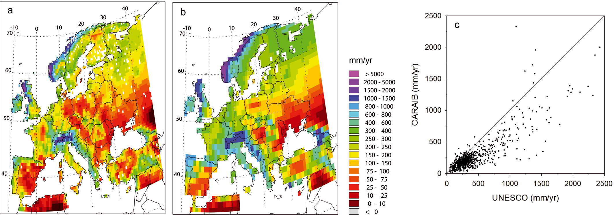
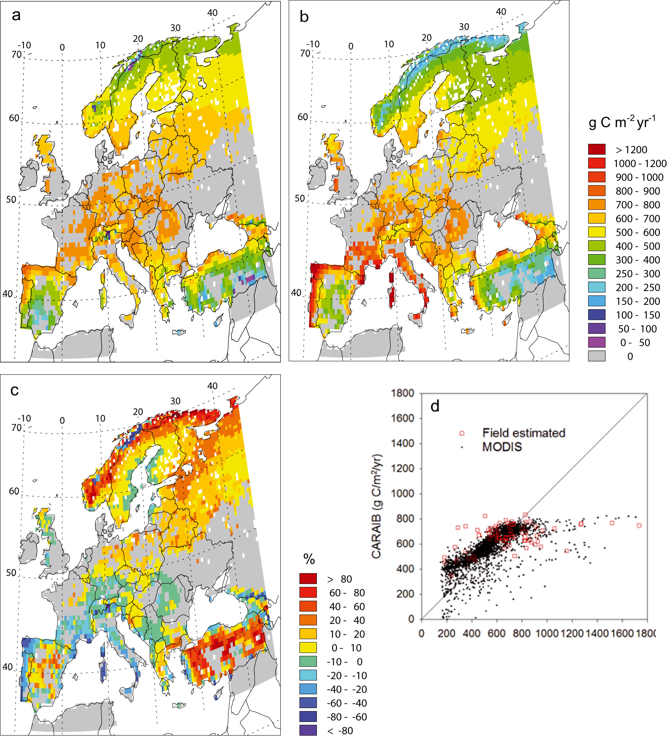
Fig. 3a and 3b compare CARAIB NPP computed values with NPP estimations of MODIS sensor for grid cells with ≥ 30 % natural vegetation. A large proportion (70 %) of the CARAIB values lies in the -20 to +20 % range of the MODIS data. The largest differences occur in the Mediterranean region where CARAIB tends to underestimate MODIS NPP values (Spain, south of France, Italy) and in the northern regions where it tends to overestimate them. A second comparison of CARAIB NPP computed values is given in Fig. 3c where CARAIB NPP is plotted versus stand-level estimates and MODIS products. CARAIB values are positively correlated with both sets of data, but CARAIB tends to underestimate the highest values and to overestimate the lowest ones. The CARAIB values are significantly higher than the MODIS estimates (t-test for paired samples = 12.91, ddl = 3080, p-value = 0.00), but with field data the difference between the mean is not significant (t-test for paired samples = 0.19, ddl = 70, p-value = 0.85).
Fig. 3 - Mean net primary productivity (g C m-2 yr-1) from: (a) CARAIB and (b) MODIS sensor for the 2000-2006 period for grid cells with ≥ 30 % natural vegetation; (c) NPP relative anomalies (%) between (a) and (b); (d) relationship between CARAIB NPP computed values and NPP MODIS estimated values for pixels occupied with ≥ 30 % natural vegetation for the 2000-2006 period (black points) or NPP field estimates collected between 1947 and 2005 (red squares - [64], [55], [79], [20], [81], [88], [43], [32], [50], [95], [11], [57], [40]). CARAIB vs. Modis data: correlation coefficient r = 0.7258, ddl = 3080, p-value = 0.00; CARAIB NPP mean = 567.0 g C m-2 yr-1, MODIS NPP mean = 536.7 g C m-2 yr-1. CARAIB vs. field estimates: correlation coefficient r = 0.4133, ddl = 70, p-value = 0.00; CARAIB NPP mean = 678.5 g C m-2 yr-1, field estimated NPP mean = 672.7 g C m-2 yr-1.
As shown by Otto et al. ([71]) for the global scale, despite the well-known problems of comparing vegetation maps due to classification and differences between actual and potential vegetations, there is generally a rather good agreement between CARAIB simulated biome distributions and other reconstructed potential vegetation distributions. Over Europe (Fig. 4), CARAIB biome distribution was compared notably with [6]. With CARAIB, Europe is mostly covered by forests, from boreal forests in the north, to mixed forests in southern Scandinavia, Russia and some mountainous areas, to deciduous forests in lowlands of Central and Western Europe, and to warm temperate (Mediterranean) forests in southern Europe and on the Atlantic coast of France. However, some problems occur, particularly on places of limited extension located on the borders of the simulated area. In the extreme north of Scandinavia, CARAIB simulates boreal open woodlands while on other vegetation maps tundra seems more widespread. In the south-west of the Iberian Peninsula, potential vegetation types are of open woodlands or of matorral types, but CARAIB produces temperate steppes. In southern Ukraine, temperate broadleaf deciduous forests are simulated while steppes are observed in most areas and are probably the potential vegetation types.
Fig. 4 - Biome distribution computed by CARAIB for the 1981-2000 period.
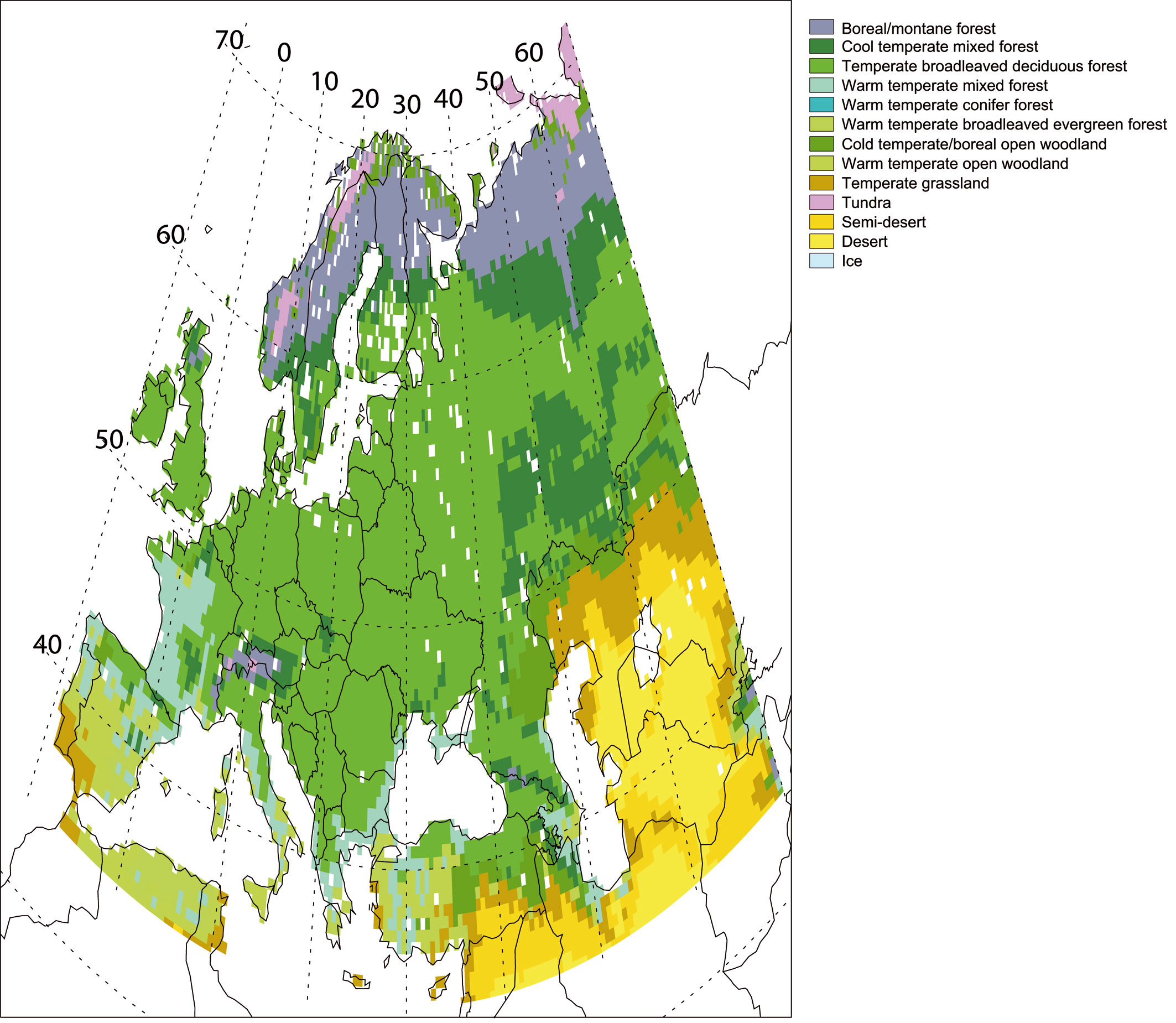
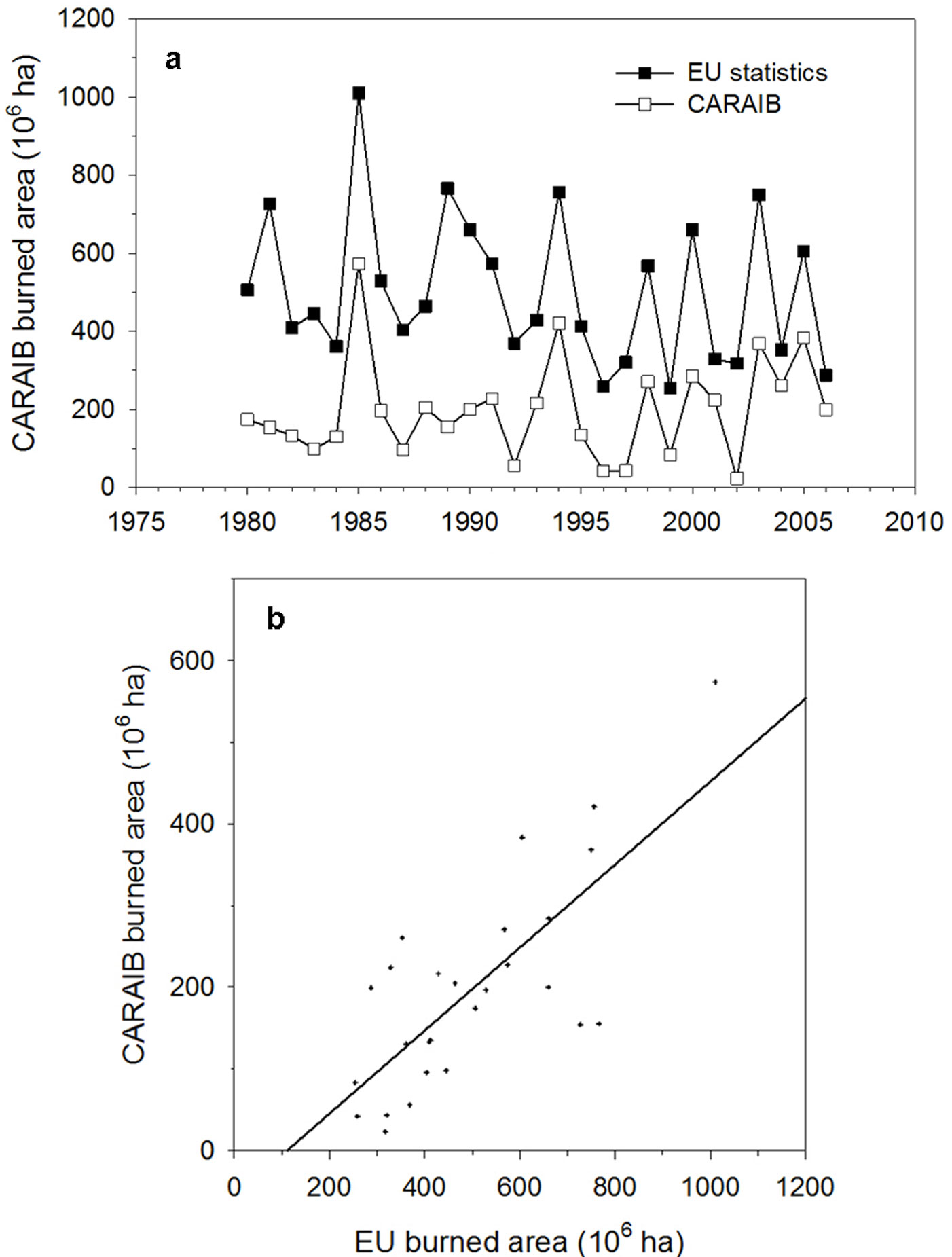
Fig. 5a shows the simulated and the observed area burned ([47]) in the Mediterranean region (Portugal, Spain, France, Italy, Greece, Bulgaria and Turkey) over the 1980-2006 period. The simulation was driven by CRU 1961-2006 climatic dataset with potential vegetation and without the human impacts (as fire ignition and fire fighting efforts). The model reproduces the observed interannual variability of fire events under specific meteorological conditions (correlation coefficient between modelled and observed values = 0.7559, Fig. 5b) but, as expected, the simulated burned area is lower due to the absence of human-induced fires.
Fig. 5 - Comparison of simulated and observed area burned (106 ha) in the Mediterranean region ([47]). (a) Evolution over the 1980-2006 period and (b) relationship (correlation coefficient r = 0.7559, ddl = 27, p-value = 0.00).
Projections over 21st century
Forced with the A2 scenario, ARPEGE/ Climate predicts substantial warming over Europe in all seasons (in average 4.3 °C increase of the annual mean temperature). Northern Europe shows a maximum temperature increase in winter (5 to more than 9 °C) while in southern Europe and in the Mediterranean region, the warming is more pronounced in summer (5 °C by up to 8 °C in the Balkans and in Ukraine). Concerning precipitations, in winter, ARPEGE/Climate predicts decreases (0-120 mm) over most regions below 50° N, except in the Caucasus and in Central Asia and increases above this latitude (0-120 mm), except in the south of Sweden (decrease of 0-30 mm). In summer, precipitations increase above 60° N (0-80 mm) while in the other parts of Europe they are projected to decrease (0-120 mm), except in Mediterranean area and in the Alps (increase of 0-40 mm). Compared with projections of other climate models from the ENSEMBLES European project ([89]), ARPEGE/Climate lies among the ones which produce the most significant temperature (warmer) and precipitation (drier) changes. The winter warming in northern Europe is particularly important while the summer temperature increase over Southern Europe is in the range of ENSEMBLES projected changes. ARPEGE produces precipitation decreases in winter over southern Europe that are more pronounced and more widespread (by up to 50° N) than those of the other climate models. In summer, the model projects very marked precipitation decrease over western (France, north of Italy) and Eastern Europe (Ukraine, Romania, etc.) and almost no change in the Mediterranean region unlike other projections.
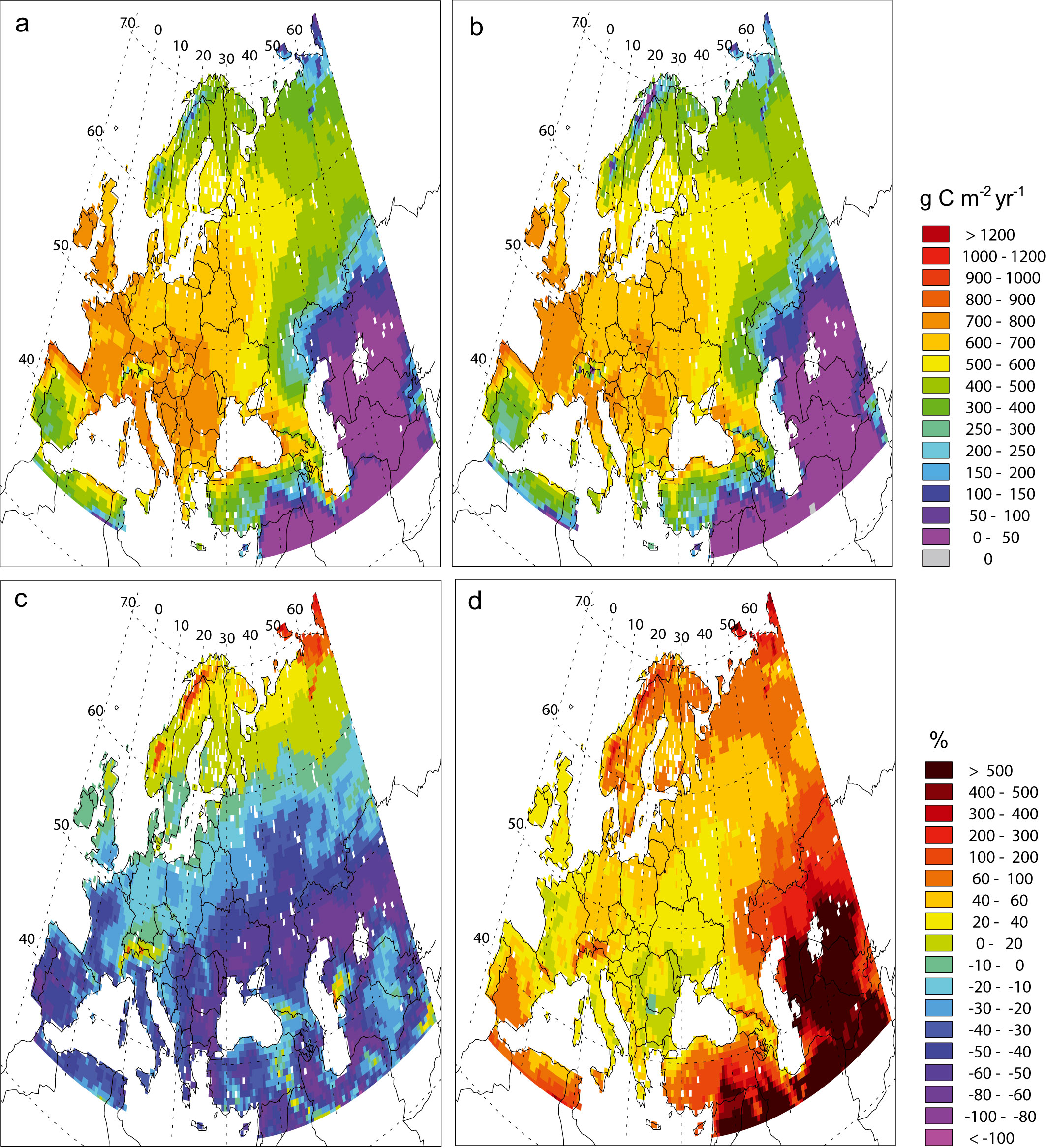
Fig. 6 presents the NPP relative anomalies under changing climate between the end of the 21st century (2081-2100) and the present (1981-2000) without or with CO2 fertilizing effect. The first simulation is driven with atmospheric CO2 concentration kept constant (330 ppmv) in the vegetation model but with climate change from A2 scenario calculated by ARPEGE/Climate. In the second simulation, the CO2 concentration is rising according to the A2 scenario in both the climate and vegetation models. The Fig. 6a and 6b display the current NPP computed by CARAIB respectively with climate from ARPEGE/Climate and CRU data. Under the first hypothesis (Fig. 6c), the NPP anomalies predicted over Europe present a large geographical gradient. Three main evolution types may be distinguished. In cold regions, i.e., at high latitudes and altitudes, the temperature increases lead to longer growing seasons. When water is not a limiting factor, plant growth is improved and thus the modelled NPP generally increases by up to 40% or even 60-100% in the coldest regions which are currently tundras. In the cold temperate area, between approximately 50° N to 60° N, NPP might decrease by as much as 50%. These NPP reductions are due to summer droughts more recurrent than in the present. In warmer regions, i.e., Mediterranean area, western France, Eastern Europe, Ukraine, south of Russia and areas around Caspian and Aral Seas, higher predicted temperatures raise evapotranspiration. Since there are no precipitation increases, plants are subject to higher water stress and NPP goes down everywhere with local decreases reaching 80%. Assuming increasing CO2 concentration together with climate change (Fig. 6d), predicted NPP increases throughout Europe, though there are substantial differences in the magnitude among subregions. As in the simulations keeping CO2 constant, at high latitudes and in mountainous areas, the model predicts NPP increases of 50-75%. For the temperate regions, the NPP increases are comprised between 25 and 50%. In the Mediterranean area, western France, Eastern Europe and Ukraine, NPP increases might reach 75%, but generally about 50%. Farther to the east, the model simulates very important increases of up to 500 %. The fact that NPP anomalies are displayed as percent makes that regions with current low NPP values (< 150 g C m-2) show the more dramatic changes. It concerns particularly south-eastern part of the studied area occupied by steppes and the extreme of northern Europe covered by tundras.
Fig. 6 - Mean net primary productivity (g C m-2 yr-1) computed by CARAIB with climate from (a) ARPEGE and (b) CRU for the 1981-2000 period. NPP relative anomalies (%) between 2081-2100 and 1981-2000 with (c) constant and (d) increasing atmospheric CO2 concentration conditions.
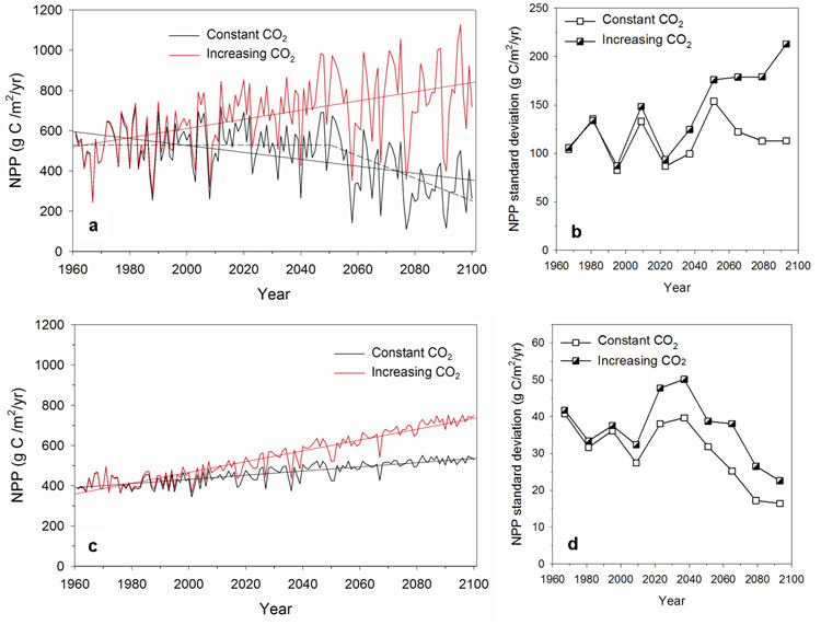
Since most climate projections indicate future changes in climate variability ([37], [38], [75]), including the ARPEGE/Climate forced with A2 scenario used in this study, the NPP variability is also studied here. A comparison of the NPP variability for the 1981-2000 period calculated with the ARPEGE/Climate model outputs (Fig. 7a) and with the CRU dataset (Fig. 7b) reveals that GCM-derived NPP may be slightly more variable than that obtained with observed climate, at least for some areas. This discrepancy between modelled and observed climate variability may affect the NPP absolute variability calculated for the future, although the trend between the present and the future may be more robust. Under constant atmospheric CO2 concentration, the NPP interannual variability increases throughout Europe except in the northern part, in the Alps and in Central Asia (Fig. 7c). In the Mediterranean region, in western France, in the Balkans, in Ukraine and in the Caucasus, the projected rises are most likely linked to the increase of the precipitation interannual variability in those regions. Between 50° and 60° N, higher temperatures probably induce more frequent water stress. At high latitudes, despite increasing NPP, variability decrease reflects reduced temperature variability and the associated snow cover spatiotemporal pattern. With rising CO2 concentration, an increase in NPP variability is projected in the same regions but it is more pronounced (Fig. 7d). It is partly due to the CO2 effects on plant physiology which increase strongly NPP during years with lower climatic stresses. The evolution and the interannual variability (standard deviation) of soil water (Fig. 8) and NPP (Fig. 9) over the 1961-2100 period are analysed more precisely for two grid cells with contrasted climate, located respectively in Greece (40°N 22°E) and in Finland (66°N 28°E). In Greece, the annual mean as well as the minimum and maximum monthly soil water values decrease progressively over the 21st century (Fig. 8a). These decreases are statistically significant (Tab. 3). Particularly after 2050, the minimum monthly soil water reaches very low values close to the wilting point (0 in the units of the figure) and the maximum value seldom exceeds the field capacity (1 in the units of the figure) meaning that the ground water reservoir would not be refilled. The analysis of the interannual variability shows significant increase in mean and maximum time series (Fig. 8b and Tab. 4). During the same period, NPP significantly increases assuming rising CO2 concentration while, under constant CO2, a negative linear trend over whole period is significant (Fig. 9a and Tab. 3). The shape of the data rather suggests that there is no trend before c. 2050 and a stronger linear decrease after. It was confirmed by an intervention analysis. An AR (1) model was necessary; the analysis gave a 2050-2100 trend of -5.60 g C m-2 yr-2 with p-value = 0.00. Moreover, by the end of 21st century, the interannual NPP variability significantly increases but only in the simulation with increasing CO2 (Fig. 9b and Tab. 4). In Finland, only the maximum monthly soil water amounts show a significant positive trend over the 21st century (Fig. 8c and Tab. 3) and none of the series shows any trend in variability (Fig. 8 d and Tab. 4). As today, drought events remain rare and winter precipitations which are projected to increase in the future in this area allow ground water to be refilled. In these conditions, NPP significantly increases under both CO2 hypothesis (Fig. 9c and Tab. 3) and its variability decrease over time only with rising CO2 (Fig. 9d and Tab. 4).
Fig. 7 - Standard deviation of net primary productivity (g C m-2 yr-1) computed by CARAIB for the 1981-2000 period with climate from (a) ARPEGE and (b) CRU and for the 2081-2100 period with (b) constant and (c) increasing atmospheric CO2 concentration conditions.
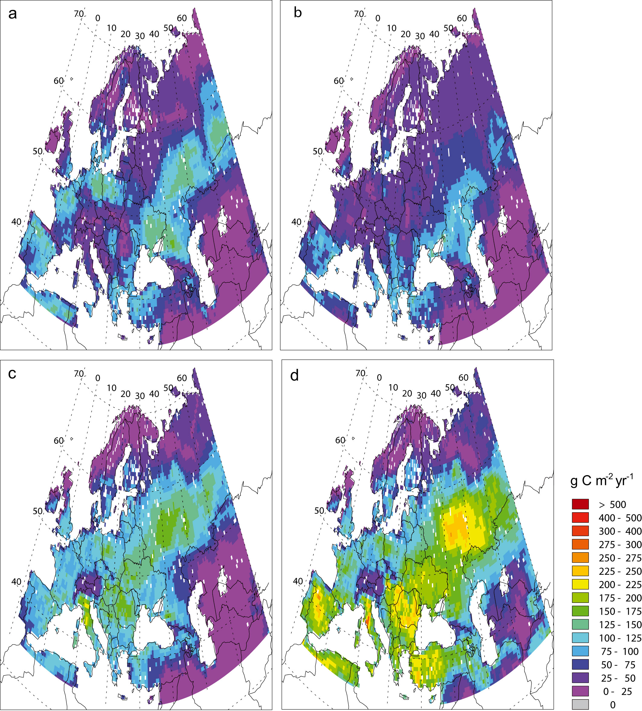
Fig. 8 - Soil water (annual mean, minimum and maximum monthly values) evolution for the 1961-2100 period and standard deviation (SD) computed by CARAIB for 14 consecutive years respectively for two grid cells in Greece (40 °N 22°E) and in Finland (66 °N 28°E). (a) evolution in Greece, (b) SD in Greece, (c) evolution in Finland, (d) SD in Finland. Soil water content is expressed in relative units, i.e., as (SW-WP)/(FC-WP) where SW, WP and FC are respectively soil water content, wilting point and field capacity in mm.
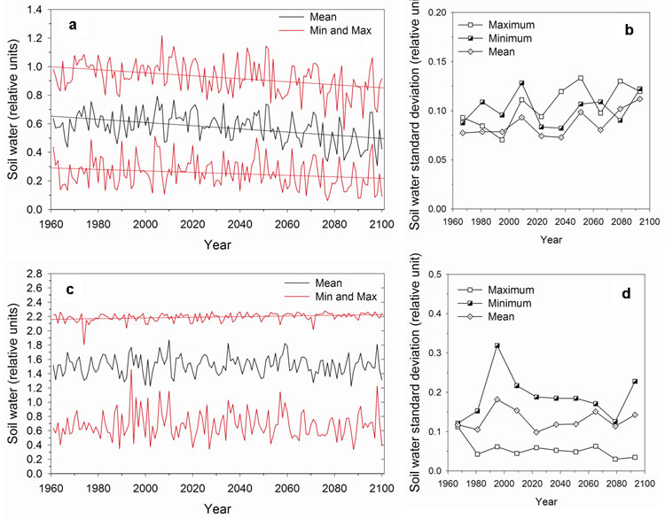
Fig. 9 - Net primary productivity (g C m-2 yr-1) for the 1961-2100 period and standard deviation (SD) computed for 14 consecutive years respectively for two grid cells in Greece (40 °N 22°E) and in Finland (66 °N 28°E). (a) evolution in Greece, (b) SD in Greece, (c) evolution in Finland, (d) SD in Finland.
Tab. 3 - Trend detection in CARAIB soil water and NPP time series. Auto-regressive (AR) and moving average (MA) effects to take into account serial dependence and p-values (significant trends (unit/yr) with *, see Fig. 8 and Fig. 9).
| Parameter | Statistics | AR | MA | Trend | p-value |
|---|---|---|---|---|---|
| Soil water in Greece | Minimum | - | - | -0.0005 | 0.02* |
| Mean | - | 1 | -0.0011 | 0.00* | |
| Maximum | 1 | 1 | -0.0011 | 0.00* | |
| Soil water in Finland | Minimum | - | - | - | 0.89 |
| Mean | - | - | - | 0.94 | |
| Maximum | - | - | 0.0005 | 0.00* | |
| NPP in Greece | Constant CO2 | - | 1 | -1.73 | 0.00* |
| Increasing CO2 | - | 1 | 2.26 | 0.00* | |
| NPP in Finland | Constant CO2 | - | - | 1.04 | 0.00* |
| Increasing CO2 | - | - | 2.68 | 0.00* |
Tab. 4 - Trend detection in variability of CARAIB soil water and NPP time series. Spearman rank coefficient (R) between time and standard deviation computed for 14 consecutive years and p-values (n = 10, significant trend with tagged with an asterisk).
| Parameter | Statistics | R | p-value |
|---|---|---|---|
| Soil water in Greece | Minimum | 0.2121 | 0.56 |
| Mean | 0.6242 | 0.05* | |
| Maximum | 0.7333 | 0.02* | |
| Soil water in Finland | Minimum | 0.1515 | 0.68 |
| Mean | 0.1152 | 0.75 | |
| Maximum | -0.4788 | 0.16 | |
| NPP in Greece | Constant CO2 | 0.1636 | 0.65 |
| Increasing CO2 | 0.7939 | 0.01* | |
| NPP in Finland | Constant CO2 | -0.697 | 0.03* |
| Increasing CO2 | -0.3576 | 0.31 |
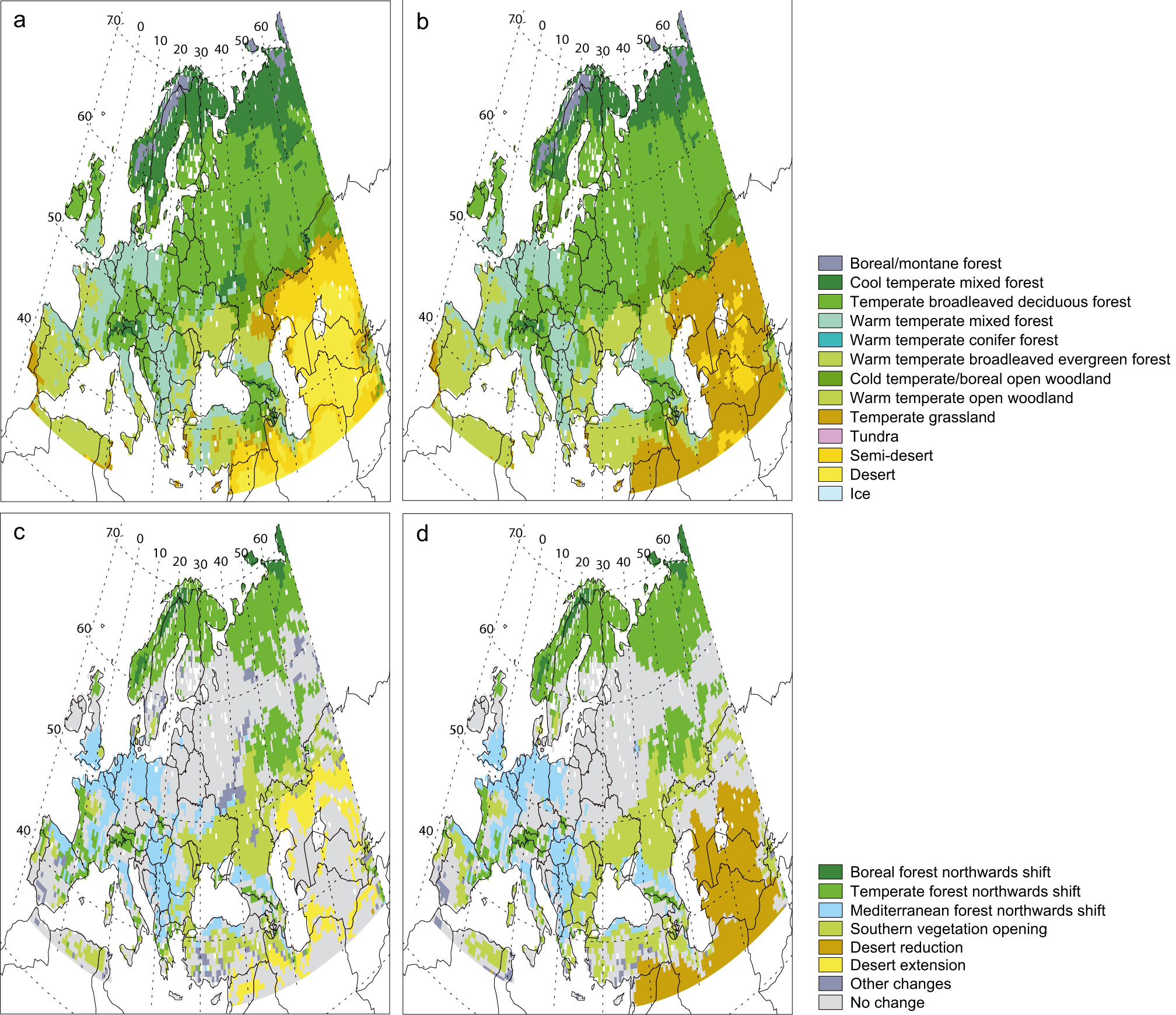
Climate change might strongly modify the vegetation distribution in Europe. With constant (Fig. 10a, c) and rising CO2 conditions (Fig. 10b, d), 54 % and 61 % of European vegetation might be respectively affected by a cover change. In southern Europe, around the Mediterranean Basin and the Black Sea, future landscape is characterized by more open vegetation. The warm temperate open woodlands expands to the detriment of temperate broadleaved deciduous forests. The Mediterranean vegetation shifts northwards, in Western and Central Europe. Temperate and boreal forests shift northwards and eastwards as well as upwards in the mountainous regions. Consequently to this tree-line displacement, European tundras might disappear almost completely and might be replaced by boreal forests. The shift from mixed forest (deciduous and conifers trees) to deciduous forest is favoured under rising CO2 conditions. The CO2 fertilization effect also limits the extension of desert areas in Central Asia by stimulating grassland development.
Fig. 10 - Biome distribution computed by CARAIB for the 2081-2100 period and biome difference map with regards to the 1981-2000 period under (a) and (c) constant and (b) and (d) increasing atmospheric CO2 concentration conditions.
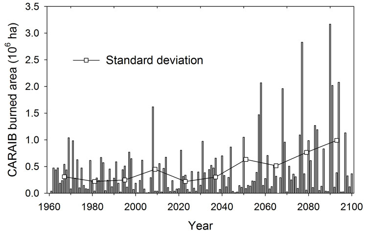
The projected climate changes over the 21st century are likely to induce increased fire risk in the Mediterranean region but also in other parts of Europe. Indeed, in the fire-prone regions, an increase in air temperature and a reduction in summer rainfall are expected, although uncertainties exist about the exact precipitation change pattern. Fig. 11 shows the burned area in the Mediterranean region (34°N to 44°N, 10°W to 40°E) over the 1961-2100 period. Trend detection was achieved with the log of the values for normalization using an AR (3) model. In those conditions no trend was detected (trend p-value = 0.37). Since the frequency distribution of the simulated area burned is log-normal, the series is probably too short to capture a future positive trend. Nevertheless, a positive trend was calculated for the variability (p-value = 0.01), which is probably the result of an increasing frequency of larger area burned fires after 2050. This increase is associated with more severe droughts after 2050 as illustrated in Fig. 8a for the grid cell in Greece. The large interannual variability in soil water might induce large fluctuations in the burned area. Wet years lead to burned area values which are comparable or lower than those calculated for the present while very dry years, occurring typically every 10-15 years, can increase burned areas by a factor of 3-5 with respect to present most severe fires. In middle Europe, up to 60°N and especially in western France, Poland, Romania, central Russia and Ukraine, fire frequency and intensity also increase significantly in the simulation. Thus, fire risks might increase almost everywhere in Europe and most countries might have to deal with likely increasing fire damages. Only Scandinavia and northern Russia might not have to face this increasing fire risk.
Fig. 11 - Area burned (106 ha) in the Mediterranean Region (34° N to 44° N, 10° W to 40° E) over the 1961-2100 period computed by CARAIB (standard deviation SD computed for 14 consecutive years).
Discussion
Model Evaluation
As outlined in the Results section, runoff is generally underestimated by CARAIB over Europe. First, though the comparison deals only with grid cells covered by more than 30 % of natural vegetation (PCLM2000 map), the simulated potential natural vegetation, predominantly forests, may lead to runoff values different than the ones observed in a landscape patterned by human land use (crops areas, asphalt areas, etc.). Secondly, some features of hydrology in mountainous area, e.g., the slope effect on runoff, are not fully represented in the model. Thirdly, CARAIB contains only one soil layer which does not allow representing the sub-surface runoff in the most appropriate way.
NPP computed by CARAIB are in the range of the estimations obtained by various methods (field estimates and remote sensing products) but the model tends however to underestimate the high productivity values and to underestimate the lower ones. Note that with MODIS, according to Turner et al. ([87]), NPP tends also to be overestimated at low productivity sites, often because of artificially high values of MODIS FPAR (fraction of photosynthetically active radiation absorbed by the canopy) and to be underestimated at high productivity sites, due to relatively low values for vegetation light use efficiency in the MODIS GPP algorithm. The discrepancies between CARAIB and data might be due to land use and management factors as well as CARAIB limitations. CARAIB produces values for non-managed mature ecosystems whereas most forest stands for NPP estimation are located in managed sites even if at the time of the studies, management have ceased. Some stands are planted with highly productive clonal selections or on former fertilized agricultural soils. For instance, a poplar plantation has the highest NPP value of 1710 g C m-2 yr-1 ([35] integrated in the [57] database) in the Fig. 3c. Stand age is also an important factor since it is established that primary productivity declines with age ([21]). Among the limitations due to CARAIB, the underestimation of runoff may indicate a bias in the water budget which may have some impacts on NPP for soil water limited ecosystems, i.e., receiving annual precipitations lower than 1500 mm yr-1 ([57]). As already mentioned, soil fertility and the influence of nutrient availability on photosynthesis and plant growth are not taken into account in the model. Moreover, the mean altitude of CARAIB 0.5° grid cells may significantly differ from stand altitude, especially in mountainous area. For instance, the Aubure site, in Vosges Mountains (France) referred with an altitude of 1000 m and a NPP of 432 g C m-2 yr-1 in Luyssaert’s database ([57]) corresponds to a CARAIB grid cell with mean altitude of only 384 m and a NPP of 689 g C m-2 yr-1. Finally, interactions with other organisms such as insects inducing partial defoliation can induce important photosynthesis decreases ([3]). This kind of disturbances is not simulated in the model which can produce overestimated NPP values.
The comparison of biome distribution obtained with CARAIB with potential natural vegetation maps underlies some problems. In Ukraine and Iberian Peninsula, the discrepancies could arise from the water budget owing to possible inaccuracy in precipitation data, in calculation of evapotranspiration or in soil data and their relationship to water conductivity. Annual runoff in these two regions is correctly calculated by the model. These regions show contrasted soil water regimes. In the Iberian Peninsula, a drought reappears every summer but winter precipitations increase soil water above field capacity and thus allow the reconstitution of groundwater stocks. On the contrary, in Ukraine, the summer drought is not so severe and recurrent, but, some years, winter precipitations are not sufficient to raise soil water above the field capacity. This can occur during two to three successive years, preventing the refilling of groundwater reservoirs. In CARAIB, tree mortality owing to water stress only begins below a fixed soil water threshold, which depends on plant type. In addition, the response is assumed quite fast (characteristic time of approximately one month). In these conditions, the model does not allow trees to survive in south-western Iberian Peninsula where the computed soil water falls below the threshold. Actually, water transfers from groundwater to the root zone should occur, especially in valley area. In Ukraine, since groundwater is not refilled trees cannot survive. It seems necessary to refine further the modelling of the vertical and horizontal dynamics of soil and ground water stocks. This kind of problem seems to appear with other dynamic vegetation models. For instance, the LPJ model also predicts deciduous trees in southern Ukraine and C3 herbs in southern Spain as dominant plant functional types ([82]). The other problem of tundra distribution in northern Scandinavia could be linked to the values of the coldest monthly mean night temperature (Tcm) or to the growing degree-day (GDD5) thresholds determined for the tree BAGs. In addition, other meteorological factors not introduced in CARAIB such as blowing ice, strong wind or snowpack extend could limit extension of tree distribution to higher latitudes and altitudes as suggested by treeline studies ([83]).
The discrepancy between simulated and observed area burned is that only natural fires due to lightning are considered in the model. Lightning causes less than 10 % of the fires, but are responsible for the largest burned areas ([23]). Since the model simulates a fire occurrence probability for the computed potential vegetation, the probability of fire ignition due to human activities is set to zero. In human densely populated areas such as Mediterranean countries, the anthropogenic ignition due to human negligence or crime is the actual main fire-triggering agent contrary to Canada, where the role of humans in igniting fires is usually small ([4]). Vazquez et al. ([91]) suggest that more than 50% of area burned in Spain is caused by negligent and intentional human-ignited fires. The simulated values are larger than the expected 10% of fire due to lightning. Indeed, in natural conditions, vegetation is continuous and fire propagation is only limited by available flammable biomass and by meteorological or topographical factors (rivers, stony areas, cliffs). In the model, those factors are taken into account by an extinguishing probability parameter set to a fixed value as a first approximation. Increasing the value of this parameter could allow considering the fire-fighting effort and consequently reducing the burned area. Nevertheless, investigations will be necessary to include topographical resolution.
Projections over 21st century
The impacts of climate change and the potential CO2 effect on NPP of European forest ecosystems have been highlighted by two simulations with different CO2 concentration hypothesis (constant and rising concentrations). The real response of ecosystem to CO2 enrichment is however a question which is still discussed. It is argued that nutrient availability could be limiting on the primary productivity ([59]). Yet, for nitrogen, results from many experimental sites lead to suppose that this is no longer the case. Owing to release of nitrogen into the atmosphere by human activities and subsequent deposition on lands, anthropogenic nitrogen sources are now controlling the carbon balance of most of the temperate and boreal forests ([58]). As a rule, the free-air CO2 enrichment FACE project results demonstrate actual fertilizing effect with C3 plants. Despite increase dark respiration with some plant species and acclimation of photosynthetic capacity (decrease of maximum carboxylation rate of Rubisco and maximum electron transport rate leading to ribulose-1.5-bisphosphate regeneration), carbon gain is markedly greater (19-46%) in C3 plants at anticipated CO2 concentration. The reasons are the stimulation of the light-saturated rate of photosynthetic CO2 uptake and the improvement of the photosynthetic use of N ([53]). Nevertheless, at some FACE sites, tree growth and NPP remain strongly limited by nitrogen availability ([25]). Here, most of the extra fixed carbon is allocated to fine roots with fast turnover and probably to exudates stimulating microbial activities to enhance N uptake. Trees alter their allocation priorities depending on growing conditions; they favour leaves, roots and mycorrhizae depending on nutrient and water availability ([74]). In addition, others nutrients than nitrogen could also induce limitations under enhanced CO2 air concentration, a situation occurring near steady-state nutrient cycle and full canopy development, i.e., when total fine root mass and leaf area index do not increase from year to year ([48]). Since the end of the eighties, the sensitivity of the Western Europe forests to nitrogen deposition is known. In densely populated countries such as the Netherlands, Germany or Belgium, the forests are often restricted to the most infertile soils. In those conditions, nitrogen deposition induces soil base cation depletion and tree nutritional imbalances ([18], [80], [94]). Otherwise, in regions where water deficit gets worse, rising CO2 concentration offsets the effects of increasing summer drought. Indeed, stomatal closure rendered possible by a higher CO2 concentration induces increased water use efficiency. For C4 plants as well as for C3 plants, significant potential for increased photosynthesis and yield at elevated CO2 concentration might result from improved water use and reduce drought stress ([33], [1], [53]). In CARAIB, CO2 concentration controls stomatal closure in combination with photosynthesis, water stress and air relative humidity, but not the physiological acclimation of photosynthetic capacity. In addition, carbon allocation between structural pools and fast decomposing organs is fixed and there is no coupling with nutrient cycles. Therefore, CARAIB with increased CO2 concentration probably overestimates NPP at anticipated CO2 concentration. Morales et al. ([65]) and Olesen et al. ([70]) obtain with LPJ DVM less marked productivity changes with a range of regional climate models under A2 and B2 emissions scenarios. They project the greatest changes in NPP in the northern European ecosystems (35-54 % increases) and smallest changes in southern Europe (only slightly NPP declines or increases). However, the balance between the two scenarios, with and without CO2 fertilization, might be definitely established only by combining the direct observation over long periods of time of tree physiology and the coupling of DVM with nutrient cycles.
In accordance with the conclusions of Mohamed et al. ([63]) and Medvigy et al. ([61]), results show that the variability of soil water and NPP might be modified by changes in climate such as precipitations or temperature. The changes in NPP variability have to be analysed together with changes in NPP values since standard deviation is affected by the mean. NPP variability is inevitably lower in regions with low productivity.
The factors expected to play the most significant role in the fire regimes during the 21st century are land-use and climate changes. The change in fire occurrence during the last decades closely reflects the recent socio-economic changes underway in many European countries, especially in the Mediterranean region, such as depopulation of rural areas, decreases in grazing pressure and wood gathering, increase in agricultural mechanization and tourism pressure, etc. ([23]). These changes in traditional land use and lifestyles have implied the abandonment of large areas of farmland, the recovery of vegetation and an increase in accumulated fuel. Nevertheless, as explained in the Material and methods section, the aim here was only to simulate the impacts of climate change on fires but not the impacts of the changes in the human factors. When ecosystems under anthropic pressure are modelled, the human-caused ignitions can be determined by the population density. Thonicke et al. ([85]) model human ignition as a non-linear function of population density, assuming that the number of events initially increases as more people settle within a previously unoccupied region but declines with further increases in population density due to landscape fragmentation, urbanisation and associated infrastructural changes.
Conclusion
In this paper, climate change impacts and potential CO2 fertilization effects on vegetation in Europe under the A2 ARPEGE/climate scenario have been illustrated through two simulations assuming constant and increasing CO2 concentration in the vegetation model. The A2 scenario was chosen because it corresponds to a rather important increase in atmospheric CO2 and thus to very substantial climate change leading to more extreme conditions for plants. The two simulations can be expected to bracket the future evolution of the system under an A2 ARPEGE/ Climate scenario, the actual path followed depending on the nutrient budget and the efficiency of the CO2 fertilization effects. Without CO2 fertilization, NPP might strongly decrease in many European areas except in the northern part. When CO2 fertilization is included, such decreases are not observed. However, in both cases, the simulated NPP shows increasing interannual fluctuations associated with more frequent and more severe summer droughts. These drier conditions might lead to an increasing fire risk and the annual burned area is projected to rise by a factor of 3 to 5 in the Mediterranean area compared to the present.
The study focused on the future evolution of vegetation represented by Bioclimatic Affinity Groups (BAGs). It shows that these BAGs will undergo significant change in productivity and eventually mortality associated with more severe and more frequent drought events in the future. Since they have a narrower bioclimatic spectrum, individual species are probably more vulnerable to climate change than BAGs. Consequently, it would be interesting to apply dynamic vegetation models at species level in order to analyse the response of a selected set of plant species to climate change. Dynamic vegetation models are indeed probably more appropriate tools to evaluate impacts of water stress on vegetation than niche-based models ([44]), especially for fully transient simulations. However, to address more fully this problem, models should incorporate a more precise description of plant response to water stress with validation on experimental or observational site data.
The response of European ecosystems to climate change has been studied assuming no dispersal limitations. The future species distribution depends, however, on the capacity of plants to migrate. Thus, the introduction of a dispersal module into CARAIB should allow studying more accurately the potential species shift and knowing if they could move fast enough to survive. This kind of question is certainly more relevant for herbs than for trees; the distribution of the latter being most of the time human managed.
Moreover, it would be worth to continue further the analysis by using the outputs of several climate models and several IPCC SRES scenarios to evaluate the uncertainties of climate projections and their impacts on future vegetation evolution. The analysis and the validation of climate model variability at the diurnal, seasonal and interannual time scales should be also carried out since climate variability at all these time scales will govern the response of plant species to climate change.
Acknowledgements
We thank Michel Déqué (MétéoFrance, CNRM, Toulouse) for providing the ARPEGE/Climate dataset and Dimitrios Efthymiadis (CRU, East Anglia) for the CRU TS3.0 dataset. Funding for this research from the ECOCHANGE integrated project (European Commission) and from the University of Liège (FSR 2010) is gratefully acknowledged.
References
Gscholar
Gscholar
Gscholar
Gscholar
Gscholar
Gscholar
Gscholar
CrossRef | Gscholar
Gscholar
Gscholar
Gscholar
Gscholar
Gscholar
Gscholar
CrossRef | Gscholar
Gscholar
Gscholar
Gscholar
Gscholar
CrossRef | Gscholar
CrossRef | Gscholar
Gscholar
Gscholar
Authors’ Info
Authors’ Affiliation
P Warnant
E Favre
M Ouberdous
L François
Unité de Modélisation du Climat et des Cycles Biogéochimiques, Université de Liège, Bat. B5c, Allée du Six Août 17, B-4000 Liège (Belgium)
Département des Sciences et de Gestion de l’Environnement, Université de Liège, Quai Van Beneden 22, B-4000 Liège (Belgium)
Laboratoire de Physique Atmosphérique et Planétaire, Université de Liège, Bat. B5c, Allée du Six Août 17, B-4000 Liège (Belgium)
Corresponding author
Paper Info
Citation
Dury M, Hambuckers A, Warnant P, Henrot A, Favre E, Ouberdous M, François L (2011). Responses of European forest ecosystems to 21st century climate: assessing changes in interannual variability and fire intensity. iForest 4: 82-99. - doi: 10.3832/ifor0572-004
Paper history
Received: Jul 16, 2010
Accepted: Dec 09, 2010
First online: Apr 05, 2011
Publication Date: Apr 05, 2011
Publication Time: 3.90 months
Copyright Information
© SISEF - The Italian Society of Silviculture and Forest Ecology 2011
Open Access
This article is distributed under the terms of the Creative Commons Attribution-Non Commercial 4.0 International (https://creativecommons.org/licenses/by-nc/4.0/), which permits unrestricted use, distribution, and reproduction in any medium, provided you give appropriate credit to the original author(s) and the source, provide a link to the Creative Commons license, and indicate if changes were made.

Web Metrics
Breakdown by View Type
Article Usage
Total Article Views: 57913
(from publication date up to now)
Breakdown by View Type
HTML Page Views: 46492
Abstract Page Views: 3238
PDF Downloads: 6334
Citation/Reference Downloads: 121
XML Downloads: 1728
Web Metrics
Days since publication: 4764
Overall contacts: 57913
Avg. contacts per week: 85.09
Article Citations
Article citations are based on data periodically collected from the Clarivate Web of Science web site
(last update: Feb 2023)
Total number of cites (since 2011): 69
Average cites per year: 5.31
Publication Metrics
by Dimensions ©
Articles citing this article
List of the papers citing this article based on CrossRef Cited-by.
Related Contents
iForest Similar Articles
Editorials
COST Action FP0903: “Research, monitoring and modelling in the study of climate change and air pollution impacts on forest ecosystems”
vol. 4, pp. 160-161 (online: 11 August 2011)
Editorials
Adaptation of forest ecosystems to air pollution and climate change: a global assessment on research priorities
vol. 4, pp. 44-48 (online: 05 April 2011)
Technical Reports
Air pollution regulations in Turkey and harmonization with the EU legislation
vol. 4, pp. 181-185 (online: 11 August 2011)
Research Articles
The impact of land use on future water balance - A simple approach for analysing climate change effects
vol. 14, pp. 175-185 (online: 13 April 2021)
Review Papers
Monitoring the effects of air pollution on forest condition in Europe: is crown defoliation an adequate indicator?
vol. 3, pp. 86-88 (online: 15 July 2010)
Research Articles
Soil microorganisms at the windthrow plots: the effect of post-disturbance management and the time since disturbance
vol. 10, pp. 515-521 (online: 20 April 2017)
Research Articles
Potential impacts of regional climate change on site productivity of Larix olgensis plantations in northeast China
vol. 8, pp. 642-651 (online: 02 March 2015)
Technical Reports
Comparison of fire danger indices in the Mediterranean for present day conditions
vol. 5, pp. 197-203 (online: 02 August 2012)
Research Articles
Contribution of anthropogenic, vegetation, and topographic features to forest fire occurrence in Poland
vol. 15, pp. 307-314 (online: 23 August 2022)
Short Communications
Upscaling the estimation of surface-fire rate of spread in maritime pine (Pinus pinaster Ait.) forest
vol. 7, pp. 123-125 (online: 13 January 2014)
iForest Database Search
Search By Author
Search By Keyword
Google Scholar Search
Citing Articles
Search By Author
Search By Keywords
PubMed Search
Search By Author
Search By Keyword


